Moscow real estate: 30 years of impressive profit

Introduction

Between 1992 and 2008, the value of Moscow real estate showed truly impressive dynamics, increasing by about 25 times (from $ 250 to $ 6,000 on average per meter), that was followed a significant correction, lowering rates to about $ 2,500 (Figure 1). It is still 10 times higher than “before time”, but is it possible to compare today’s nominal prices and prices of the distant past? Is it possible to draw at least some conclusions from these dynamics and answer two eternal questions of any financial asset - how high or low, based on historical record, is its current value, and what is its real expected return?

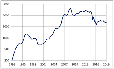
Figure 1. The average price per square meter of residential real estate in Moscow (US dollars)

Source: author’s plotting

A traditional approach to solving this problem would be to bring the initial price data to real values ​​cleared of inflation and the subsequent search for an equilibrium price using multiple regressions. However, such an approach meets many obstacles. Firstly, it is not clear in what currency to calculate, especially in light of the fact that the consumer price index in rubles, due to the period of hyperinflation, may contain critical errors, while the similar dollar index is fatally different between Russia and the United States. Secondly, during this period there is no clarity with the explanatory variables - they are either not defined as the mortgage costs, or they set heartbreaking records.

Investors need a much easier concept. Such one, that the events of the 1990s fit into its framework rather as an everyday occurrence than as an accident. The article shows that such a concept can be built on the basis of the national capital model proposed by T. Piketty [2] (Piketty, 2014). In accordance with it, the total housing stock value in Moscow is related to its GRP, which leads to the most effective separation of pricing factors into fundamental (stable) and cyclical (speculative). At the same time, GRP is counted by purchasing power parity (hereinafter referred to as GRP PPP), this is the only way to take into account quotes in US dollars, as well as to reach the equilibrium price in the form of an almost horizontal line.

Estimation of expected real returns also requires conceptual role. The widespread opinion is that investments in residential real estate are not interesting only because the rental rate is lower than the bank deposits rate, but this is fundamentally wrong. Adequate comparison of various assets requires taking into account all profitability components, and in real terms. For bank deposits, this is the nominal rate minus inflation; for real estate, the rental rate plus the long-term rise of the real price. Experience of developed countries shows that the mean historical returns of any savings tools, including bank deposits, stay near zero, while real estate gives the highest capital growth on a par with stocks [2] (Jorda et al., 2017).

However, past results do not guarantee future ones, especially for a single city, where rental rates and equilibrium values ​​may differ significantly from the described average values. In a similar situation, the only way to determine the expected real return is direct modeling of its components, which is done in this article. Thus, the long-term appreciation is represented as the averaged change in the equilibrium price exclusive of depreciation, and rental rates are calculated on the condition that the total pure rent, including imputed rent, makes constant 10 % of the official GRP. Standard deviation calculations are performed using the R/S analysis.

The rest of the article is structured as follows. The second chapter provides a brief overview of the literature. The third examines the basics of pricing and equilibrium price models, as well as the standard deviation. The fourth chapter is devoted to calculating the real expected return. The fifth chapter proposes key conclusions.

Literature overview

There are many studies on pricing in the residential real estate market, mainly in the United States market. However, these studies do not provide comprehensive answers to the above questions. Unlike equity markets, investors do not have such efficient and at the same time simple indicators as the price-earnings ratio and the ratio of the total value of non-financial corporations to GDP (known as the Buffett indicator). There are also no models for assessing current expected returns taking into account rents, while the available retrospective data obtained not by direct measurement in the image of the book “The Triumph of Optimists” [3] (Dimson et al., 2002), but indirectly, raise many questions. However, the main achievements of researchers in this market need to be mentioned.

In particular, researchers note that housing accounts for most of the property of those who own self-occupied apartments or houses. T. Piketty [1] (Piketty, 2014) combines data on the main economies of the world, showing that the total value of residential real estate in the current era is about half of national capital or 200-300 % of GNI (Gross National Income), and net rent [1] (ordinary and imputed) 7–10 % of GNI. All national capital, depending on the country, is 400-700 % of GNI, and this value, with the exception of the period in the middle of the 20th century, has been holding at the same level for the third century, setting a similar trajectory for the rent. The situation in Russia differs from the rest of the world only in details [4] (Novokmet et al., 2017). There the entire national capital is a bit smaller, and dwellings make up a larger share of it.

The initial pricing data for the real estate market can be of two types. This is the average cost per square meter, according to the Russian Federal State Statistics Service and the Administration of IRN.ru, and various indices that take into account the moral and physical aging of existing real estate. According to this scheme, the most famous Case-Shiller index in the USA is calculated. These indices are calculated by the hedonic regression method or at the prices of repeated sales of the same objects [5] (Case, Shiller, 1987). They, of course, show worse dynamics than the average price per square meter. Nevertheless, in the long run, they still overtake the consumer price index, providing real profitability in addition to the rent.

R. Shiller (2005) shows that since 1890, US residential real estate has risen in price at an average rate of 0.4 % per year, but in recent decades, the growth rate has accelerated markedly. Other researchers [7] (Knoll et al., 2014) note that the tendency to rise in price is also observed in other developed countries. Moreover, for the period after the end of World War II, the average growth rate for a sample of 14 countries is about 2 % per year. The authors of the study emphasize that 80 % of this increase is due to higher land prices and only 20 % due to increase of construction costs. The turning point in the global trend, as a result of which the sideways trend of the first half of the 20th century gave way to steady growth, is associated by researchers with the end of the transport revolution and growing restrictions on land use.

Efficiency of the real estate market has been called into question since the pioneering work of Case and Shiller [8] (Case, Shiller, 1988). Their followers, for example Gao [9] (Gao et al., 2009), show that inertia is inherent in residential real estate prices, also known as momentum, but at the same time they have the feature of mean reversion. This means that the rise or fall in prices in the current year is likely to continue in the next year, however, as you move away from the market equilibrium, the likelihood of a return to it will increase. Determining the equilibrium price using multiple regressions, Gao and others confirmed a significant overvaluation of US residential real estate on the eve of the mortgage crisis, but their experience for the above reasons is only suitable for developed markets, not for Russian realities.

The total geometric mean return on investment in real estate, including depreciation and operating costs, since 1950 has exceeded 7 % [2] (Jorda et al., 2017). This value is calculated indirectly, on the basis of rent indices and the actual price of housing, which allows for very significant errors compared to what investors could actually get. However, the authors insist on their own and confirm the accuracy of the calculations by comparing them with other sources, in particular, with the results of real estate trusts. The rental rate is more than 5 %, but this is an average value, not indicative of a particular city. For example, for Paris, the current rate is only 3 % [1] (Piketty, 2014).

Two domestic monographs by Sergey and Gennady Sternikovs [10, 11] (Sternik, Sternik, 2009; Sternik, Sternik, 2018) shall be distinguished from domestic works. The authors show that at present the Russian real estate market (including the Moscow market) is already quite mature. Therefore, the main obstacle to its analysis is the depth of the data, but not the individual characteristics. But the authors' methods have one significant drawback, they consider real estate prices in the context of such extremely unpredictable factors as supply and demand, and therefore their results are really useful for understanding only the past and present, but not the future. Long-term forecasting is only possible scenario-wise, but this does not suit many investors.

The model of national capital

How to find out how expensive or cheap an asset is? The trivial way is to determine the equilibrium price and compare it with the current price. All pricing factors, in addition to inflation, are divided into two groups: fundamental (stable), which are responsible for the equilibrium drift and, therefore, for the return on the asset, and cyclical (speculative), which are responsible for fluctuations and attractiveness of the current price based on historical comparisons. The first group of factors, such as the size of the population or its disposable income, change extremely slowly and leave their trajectory only under the condition of political upheaval, while the second group, investor sentiment and even the cost of the mortgage, simply fluctuate with or without the business cycle.

Since construction, due to land deficit and restrictions on its use, is not able to satisfy the growing needs of society, the equilibrium price should be sought only on the basis of demand patterns. The simplest of them is a continuation of the concept of national capital by T. Piketty [1] (Piketty, 2014) and involves a comparison of the total value of the housing stock in Moscow and its GRP. The interpretation of this model is very simple - GRP sets the total income of the region's residents and, therefore, the amount of money that they are able to spend on paying rent - ordinary or imputed. And all these funds account for the total volume of housing available, while new construction affects only the drift of prices. The formula for calculating the relative value of the housing stock (g) is as follows:

, (1)

where A is the total housing stock in Moscow, E is the average price per square meter (in US dollars), and GRP is the GRP of Moscow (in US dollars at the official rate).

The value of E is taken according to the website IRN.ru [2] and is a marginal plausible valuation of the average market (in US dollars) price per square meter in the secondary market, which is ideal for determining the housing stock value, but this turns out not to be enough. It can be seen from the above formula that the ruble exchange rate is implicitly contained in both the numerator and the denominator, and therefore, after its reduction, all final prices will be taken into account in rubles, which contradicts the original idea of clearing the Russian currency rate fluctuations. The graph based on this formula (Figure 2) is also not distinguished by verisimilitude, since the value of housing, that reached in the 90s above 400 % of GRP, based on the experience of other countries, is too large.

A possible explanation for the phenomenon of the 1990s is that in conditions of hyperinflation, investors focused on some fair assessment of their rental income, and not at all on the basis of the extremely low ruble market rate. If so, then the only way to find market equilibrium is to use, instead of the usual GRP, the corresponding value for purchasing power parity that, by convention, will not be connected in any way with the exchange rate of the Russian currency. Now, as required, all prices are taken into account strictly in US dollars, and the final chart (Figure 3) visually represents fluctuations around a slowly growing line, which corresponds to the global trend. The mean value of 140 % is natural, since the GRP by PPP of Moscow is typically larger than the usual GRP.

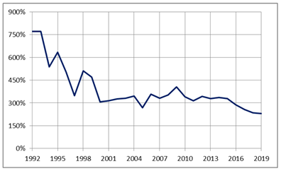
Figure 2. The housing stock value in Moscow as a percentage of GRP [3]

Source: author’s plotting

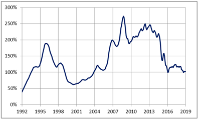
Figure 3. The housing stock value in Moscow as a percentage of the GRP by PPP

Source: author’s plotting

It is worth mentioning that due to significant inequality between Moscow and the rest of Russia, the so-called Penn effect must be present in their economies. This means that the price level in the GRP of Moscow (the ratio between GRP and GRP by PPP) will be slightly higher than the similar value for the country as a whole. Assuming that the logarithm of the price level and the logarithm of GDP per person are linearly linked with a coefficient of 0.242 [12] (Cheung et al., 2016), the total GRP by PPP of Moscow (PPP_M) can be estimated by the formula:

(2)

where PPP_R is GDP by PPP of Russia, d is the share of Moscow in Russia's GDP, and k is a measure of inequality (the ratio of GDP per capita between Russia on average and Moscow).

The standard deviation based on monthly IRN data is 11 %, while on the basis of annual data it is already 24. This is because the values ​​used in the calculations are not the closing prices of exchange trading, but some mean values ​​obtained after noise removal. Also due to illiquidity the initial impulses to increase or decrease are played out in price for more than one month. The Hurst indicator for the trend-free ratio of housing value to GRP by PPP, calculated with the simplified formula [13] (Hurst, 1951), is 0.8, which differs significantly from the values ​​0.58 – 0.68 obtained by Peters [14] (Peters, 1996) for the main assets traded on the exchange. The expression for the Hurst coefficient (H) is written as follows:

, (3)

where R is range, S is standard deviation of return, and n is number of measurements.

A study on the MSCI index showed that measurement of standard deviation of return based on annual average data underestimates its true value by 1.14 times [2] (Jorda et al., 2017). If this coefficient is applicable to Moscow real estate, then its standard deviation is 27 %. But there is another way. Namely, to assume that the magnitude of the ratio of the housing stock value to GRP by PPP, measured by the extreme values ​​of 2008 and 1992, is true, whereupon the ratio can be simply attributed to such a standard deviation at which its Hurst indicator is 0.63. From here, it again turns out to be 27 % and this only confirms the legitimacy of previously made assumptions.

Actual expected return

How to calculate the current expected return? For stock markets, where there is a lot of historical statistics, this problem is excellently solved. In particular, such a decision is given in the book “The Triumph of Optimists” [3] (Dimson et al., 2002). However, this is not our case, since for Moscow real estate no such statistics exist neither in terms of rental rates, nor in terms of re-sale indices. Therefore, the only way to determine the current expected return is to analyze its components individually, based on cross-country comparisons. By definition, the expected real return (e) is:

(4)

where r is net rental yield, b is long-term rise in price per square meter, and Δb is losses due to aging.

Net rental return is the rental rate minus operating costs that include utilities, repairing, depreciation of the apartment furniture and equipment, as well as insurance. The rental rate is calculated according to the website Domofond.ru, which shows the average (per meter) offer prices (for rent and for sale) based on ads on the Internet, while all operating costs are simply assumed to be 1.5 %, this is the average value for those developed countries with rich historical statistics of national accounts [2] (Jorda et al., 2017). Unfortunately, such estimates are very inaccurate, and the Domofond.ru series is also too short (since December 2013), however, they nevertheless allow us to establish the fact that net rent, like other countries, has almost a constant (10 %) share of ordinary GRP, from where:

(5)

where g is the ratio of the housing stock value to ordinary GRP.

The long-term real appreciation of a square meter is the profitability that accumulates during a year with the ratio of the housing stock to the GRP by PPP remaining constant. Obviously, it is formed due to the fact that the real GRP by PPP, moreover deflated at international rather than domestic Russian prices, is growing faster than the volume of the housing stock. Since 1992, this rise in price amounted to 2.5 times, which corresponds to a geometric rate of 3.45 %. But this is again past data, which, among other things, reflects a huge jump in the share of Moscow in Russia's GDP due to migration and growing inequality between the capital and the regions. Thus, the population of the capital during this period increased by 40 % against a fall of 1 % in Russia, while the real GRP per capita by PPP grew by 2.68 times against the growth of 58 % in the country as a whole.

Moreover, this rise in price has never been uniform in history. In fact, it completely fell within a single decade from 1999 to 2008, so the graph (Figure 4) resembles a logistic curve rather than a sequential rise. In recent years, certain stagnation has taken shape in the Russian economy, as a result of which all long-term appreciation has become a thing of the past, but investors should hope that these difficulties are temporary due to a downward wave of the commodity cycle [4]. If you imagine that real world GDP per capita will continue to grow at a rate of 1.6 % per annum (average rates over 50 years), and Moscow’s living standards will not change relative to world standards, then, while maintaining the same pace of construction and population growth, a long-term rise in price will be 1,2 %.

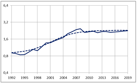
Figure 4. Long-term rise in price per square meter in Moscow [5]. The solid line is the calculated value, the dotted line is the approximation

Source: author’s plotting

The last component is the correction for moral and physical aging of the structure. It is divided into two parts – depreciation of investor-owned real estate and “losses” due to new construction, which in fact erodes its share of the total housing stock. But the construction has already been taken into account earlier, while depreciation can be calculated using the obvious assumption that the “average” real estate has been operated for exactly 75 years, after which only the land under it remains in the ownership of the investor. Given that the construction share in Moscow accounts for no more than a third of the initial cost of such an object, the adjustment for depreciation is a modest 0.5 % and, therefore, it is permissible to simply “hide” it in operating costs that are clearly overestimated from the point of view of Russian specifics.

The graph of the real return is shown in Figure 5. When plotting it, it was taken into account that the net rent clearly depends on the current price, while long-term appreciation is not associated with it, and therefore, in order to exclude the appearance of full return in negative territory, and at the same time to underscore rental rates, the second component (b value) was calculated based on the logistic curve. But the goal was only partially achieved, since the real rise in price still retains its dominant influence, hiding even a significant drop in rental rates of the 1990s, which occurred as a result of the understated ruble exchange rate. But most of all, the chart is striking in the fact that the peak of expected real return in 2002 accounted for exactly the significant bottoms of the market. Where investors looked, remains a big mystery.

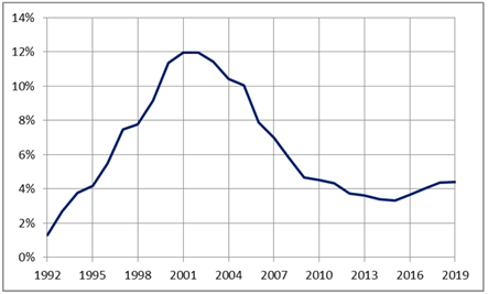
Figure 5. Expected return on investment in Moscow real estate

Source: author’s plotting

Conclusion

In comparison, the current expected return on Moscow real estate (4–5 %) is close to the corresponding values ​​for the United States stock market and Paris real estate market [6]. In this case, the standard deviation is much larger, but it is probably overestimated due to the presence of a long stage of political instability and, in addition, is offset by an underestimation relative of the equilibrium price, which is a rarity for the modern world mired in quantitative easing. If so, then the current characteristics of Moscow real estate are quite interesting, although the expected return is clearly inferior to the realized historical one, which, if rent could be reinvested, could amount to 8.4 % unrealistic for modern markets.

But this is only a theory, since in preparing the calculations, as in other similar works, many dubious simplifications were made. In particular, taxes, which always differ for different categories of investors and therefore are not reduced to any uniformity, were not taken into account. The description of operating costs as a percentage of the value of the object is very superficial, and the issue of land ownership under the houses, presented as resolved in favor of homeowners, actually hangs in the mid-air. In addition, transaction costs, downtime of facilities and all other subtle gaps through which a part of the profit always leaks were not taken into account. The investor will have to take into account all these “subtleties” on his own, but he will be armed with the technique proposed in this article.

Another fundamental conclusion is that full-fledged private property relations in modern Russia have developed in just a few years, and that they foredoomed the country's exit from the post-Soviet crisis, but not the other way around. At the same time, residential real estate was actually the only tool with which Soviet citizens could carry savings through a series of financial shocks, including monetary reform, hyperinflation and default. Price recovery was quick enough every time, so the first bubble in the Moscow market was inflated already in the 95th year. In this case, the equilibrium value was repelled from the actual product being produced, ignoring the ruble exchange rate, so that the property could not only be held until the “best times”, but also sold at a good price.

[1] Data on net rents are only for France and the UK.

[2] Details of the method can be found on the website: https://www.irn.ru/methods/

[3] The value for the 1992th year, in fact, is not defined and taken equal to the value for the 1993th year.

[4] The author’s forecasts based on Kondratiev cycles can be found in the article “The History of Energy Prices” published in the journal Economic Strategies. 2018, No. 1.

[5] The displayed value is the real GRP by PPP of Moscow (billions of chained 2011 dollars) per million square meters of total housing stock.

[6] Data for Paris is provided by Friggit, J. (2002). “Long Term Home Prices and Residential Property Investment Performance in Paris in the Time of the French Franc, 1840–2011” and in other materials on the website

http://www.cgedd.developpement-durable.gouv.fr/

References:

Case K., Shiller R. (1988). The Efficiency of the Market for Single Family Homes NBER Working Paper № 2506.
Cheung Y-W., Chinn M., Nong X. (2016). Estimating Currency Misalignment Using the Penn Effect: It`s not as Simple as it Looks Working Paper № 22539.
Dimson E., Marsh P., Staunton M. (2015). Triumph of the Optimists. 101 Years of Global Investment Research Princeton University Press.
Gao A., Lin Z., Na C. (2009). Housing market dynamics: Evidence of mean reversion and downward rigidity Journal of Housing Economics. (18). 256-266.
Hurst H. (1951). Long-term Storage of Reservoirs Transactions of the American Society of Civil Engineers. (116). 770-799.
Jorda O. (2017). The Rate of Return on Everything, 1870–2015 FRBSF, Working Paper. (25).
Knoll K., Schularick M., Steger T. (2014). No Price like Home: Global House Prices, 1870-2012 FRBD Globalization and Monetary Policy Institute, Working Paper № 208.
Novokmet F., Piketty T., Zucman G. (2017). From Soviets to Oligarchs: Inequality and Property in Russia 1905-2016 NBER Working Paper № 23712.
Peters E. (2000). Khaos i poryadok na rynkakh kapitala [Chaos and order in capital markets] (in Russian).
Piketti T. (2016). Kapital v XXI veke [Capital in the twenty-first century] (in Russian).
Shiller R. (2017). Irratsionalnyy optimizm [Irrational optimism] (in Russian).
Sternik G., Sternik S. (0). Metodologiya modelirovaniya i prognozirovaniya zhilischnogo rynka [The methodology of modeling and forecasting of the housing market] (in Russian).
Sternik G., Sternik S. (2009). Analiz rynka nedvizhimosti dlya professionalov [Market analysis for real estate professionals] (in Russian).