Estimation of the monetary policy impact on the Russian macroeconomic indicators

1. Introduction

This article is devoted to modelling the effect of variables utilized in the Bank of Russia’s monetary policy, i.e. monetary base and money supply, on key indicators of Russian economic development: GDP, customer price index and the rouble real effective exchange rate. As the theoretic basis for this work, the article by K.N. Koritschenko “Contradictions between the Budget and Monetary Policies in the Modern Russia as the Main Cause of Crises” [O protivorechii byudzhetnoy i monetarnoy politiki sovremennoy Rossii kak osnovnoy prichine krizisov] was taken. Based on this article, the main hypotheses that were formed will be further checked statistically. Let us list them in short.

Hypothesis 1. Variables of the Bank of Russia’s monetary policy (money supply and monetary base) have statistically significant effect on GDP growth rates.

Hypothesis 2. Variables of the Bank of Russia’s monetary policy (money supply and monetary base) have statistically significant effect on the rouble effective exchange rate.

Hypothesis 3. Variables of the Bank of Russia’s monetary policy (money supply and monetary base) have statistically insignificant effect on the inflation rates.

2. Data

Like the statistic basis for the following study, the data series bellow with indication of the source and the format were used:

· Gross domestic product in constant prices of 2008 (the data of the Federal State Statistics Service): Quarter data since the 1^st quarter of 2002 to the 4^th quarter of 2014.

· Monetary base in broad definition (data of the Bank of Russia): Monthly data since January 2002 to February 2015 and the quarter data since the 1^st quarter of 2002 to the 4^th quarter 2014.

· Money supply (the national definition) (data from the Bank of Russia): Monthly data since January 2002 to February 2015 and the quarter data since the 1^st quarter of 2002 to the 4^th quarter 2014.

· Nominal US dollar rate to rouble at the end of the period (data of the Bank of Russia): Monthly data since January 2002 to February 2015.

· Index of the rouble real effective exchange rate to foreign currencies (data from the Bank of Russia): Monthly data since January 2002 to February 2015.

· Consumer Price Index (data from the Federal State Statistics Service): Monthly data since January 2002 to February 2015.

To erase the seasonal effects, all the eight data series (taking into account monthly and quarter data for both the money supply and the monetary base to be different series) were brought to the format “the growth rate in relation to the relevant period (month/quarter) of the previous year”. Moreover, following the results of such transformation, the issue of non-stationarity of the data series under review is closed (which was proven by the Dickey-Fuller test’s results). However, this is the reason why the modelling bellow was performed the data starting since 2003, due to the data of 2002 being used as initial values. The dynamics of the indices presented in Figures 1 to 4.

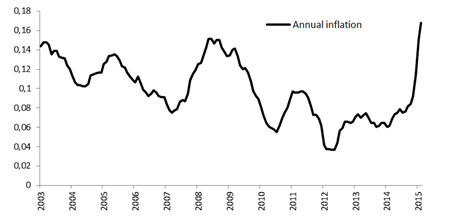
Figure 1. Inflation in relation to the relevant month of the previous year

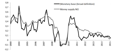
Figure 2. The growth rate of the monetary base and money supply M2 in relation to the relevant month of the previous year

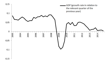
Figure 3. The GDP growth rate in relation to the relevant quarter of the previous year

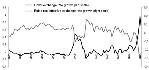
Figure 4. The growth rate of the dollar exchange rate and the rouble real effective exchange rate in relation to the relevant month of the previous year

Pay attention to several main characteristics of the diagrams provided. At first, please be aware of a major similarity between the growth rates of monetary base and money supply M2 (in Figure 2), even taking into consideration the fact that the money supply exceeds the monetary base by two or three times (depending on the reviewed year). If we split the money supply M2 into two parts – the monetary base and other M2 components – we can see that both indicators behave in a more volatile way than their sum. Thus, we can mention some mechanism that transmits the effect of the monetary base to the money supply taking into account certain compensatory effects.

Figure 4 vividly illustrates the existing relation between the dynamics of the dollar exchange rate and the rouble effective exchange rate index. As implied by the name of indicators, their movements must be opposite as adjusted to the changes in rates of other currencies and inflation in Russia and trade partner countries.

Figures 1–4 very distinctly show the leap of 2008–2009 related to the global financial and economic crisis which had the impact on the Russian economy. The next quick change happened during the second half of 2014 and, as it took place at the end of the reviewed time period, it managed to be reflected only in Figures 1 and 4.

3. Modelling

We will use the estimation of regression equations as an instrument to test the hypotheses formulated above, which use GDP growth rates, rouble effective exchange rate and consumer price level as explainable variables, and growth rates of the money supply and the monetary base as the explanatory variables, as well as, for some models, the growth rate of the nominal dollar exchange rate. It should be noted that not only current but also lagging values were used for explanatory variables up to the year (i.e. 4 periods for the quarter data and 12 periods for the monthly data). Such an approach allows estimating not only the level of effect but also the lagging of the effects in time (the depth of the so-called “transfer effect”).

After estimating the model containing all explanatory variables that are possible in this case and taking into account the testing of residues for normality (the standard Jarque-Bera test), the variables that are insignificant at the 10% level of significance were excluded. This measure was repeated until all residual variables in the model had p-value less than 10%. Note that, despite the significance level, this rule was never applied to the constant that had always been in the model. The model obtained through this method was submitted to testing for the presence of residual autocorrelation by the Durbin-Watson test. Furthermore, we won’t be explaining these technical issues in detail, assuming that the final equations were fully obtained according to all the above mentioned.

We should mention the use of the lagging value models of the explained variable separately, i.e. of addition of the autoregressive part in the regression equation. This practice is rather popular in the field of econometric studies, but we will use it only if the procedure described above happens to not provide any acceptable results. Unlike the accepted practice, this caution is connected to the initial task, not only to describe the dependencies between variables on the retrospective data, but also to create an instrument suitable for forecasting more than one period forward.

3.1. The GDP Growth Rate

According to the results of estimation the following correlation was obtained:

In this correlation the GDP growth rate is related to the relevant quarter of the previous year, is the growth rate of the money supply M2 in relation to the relevant quarter of the previous year, is the growth rate of the monetary base in relation to the corresponding quarter of the previous year. Here and further, the standard deviation of the relevant index estimation is given in round brackets, under the index. The quality of the model is provided in Figure 5 ().

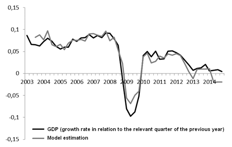
Figure 5. GDP model estimation in relation to the relevant quarter of the previous year

It’s visible that the model quality’s high characteristics are the result of not only the correct description of rapid changes in the critical years 2008 and 2009 but also due to the correct description of the dynamics before and after this period of time.

Please be aware that the equation includes only lagging indices of the money supply and the monetary base which can be used for determination of the cause-and-effect link in this set of indicators. The equation includes two variables with the lag of one quarter, notably the negative index stands before the growth rate of the monetary base. Nevertheless, it doesn’t mean that the growth of monetary base slows down the GDP growth. The point is that for most of its components, the monetary base is included into the greater aggregate – the money supply. In this sense, in order to obtain the approximate (as we actually speak of rates, not of sums) index of the monetary base effect, one must add up indices for these variables, i.e. 0.341. In its turn, 0.495 is the index with which the growth rate of other M2 components influences on the GDP growth rate. At last, pay attention to the negative index before the growth rate of the money supply two quarters earlier. As far as it can be seen, it refers to some compensation for the effect of this variable in time. In general, hypothesis 1 described above is not rejected at the econometric level.

3.2. Rouble real effective exchange rate

Based on the results of estimation of the regression equation for the growth rates of the rouble real effective exchange rate, the following correlation was achieved:

In this correlation is the growth rate of the rouble real effective exchange rate in relation to the relevant month of the previous year, is the growth rate of the dollar rate in relation to the relevant month of the previous year, is the growth rate of the money supply M2 in relation to the relevant month of the previous year, is the growth rate of the monetary base in relation to the relevant month of the previous year. The quality of the model is shown in Figure 6 ().

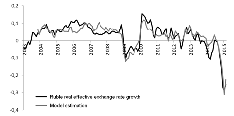
Figure 6. Model estimation of the growth rate of the real rouble effective exchange rate in relation to the relevant month of the previous year

It’s important to realize that the presence of the growth rate of the dollar exchange rate is mandatory for the correct calculation of the effect of monetary factors on the growth of the rouble real effective exchange rate. When analysing the obtained equation, attention should be given to the time distribution of the effect of money supply and monetary base on the rouble real effective exchange rate. We certainly see that the variables of the Bank of Russia’s monetary policy (the money supply and the monetary base) cause a statistically significant effect on the rouble effective exchange rate, i.e. hypothesis 2 is also not rejected. However, this effect should be considered as a relatively short-term one. As we can see in Figure 2, the growth rates of money supply and monetary base are rather similar, so we can compare the indices in the present correlation. The sum of indices before all the lagging variables of the money supply and the monetary base is very close to zero. This means that 10 months later the effect of monetary factors on the real rouble effective exchange rate is mutually compensated.

3.3. Consumer Price Index

Given the estimation results of the regression equation, the following correction was obtained for the consumer price index:

.

In this correlation, is the growth rate of the consumer price index in relation to the relevant month of the previous year, is the growth rate of the dollar rate in relation to the previous year, is the growth rate of the money supply in relation to the relevant month of the previous year. The quality of the model is shown in Figure 7 ().

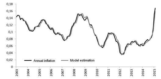
Figure 7. Model estimation of the consumer price index in relation to the relevant month of the previous year

As distinct from the two previous models, the selection of the functional form for the correlation describing inflation proved to be more difficult. The approach used before, which is based on the gradual exclusion of the growth rates of the money supply, the monetary base and the dollar rate up to the 12 month lag, didn’t present any appropriate results. Regardless of the sequence of variables exclusion, the explanatory power of those models proved to be extremely low. At first, due to that fact, we had to refuse using the growth rate in relation to the relevant period of the previous year and to use the growth rate relatively to the previous month. Unlike other variables, the clearly expressed seasonal component is not characteristic for the dollar rate, so this operation is pretty much correct. Secondly, we had to add in the model the auto-regressive part of the first order that takes into account inertia of the index.

Regarding this subject, we should separately speak about the interpretations of the ratio indices for the consumer price index. Allow us to imagine the situation in which in some month (we will further consider it to be the first and to trace down all further events from it) the money supply increases by 1%. From the viewpoint of the the index that we used in the model, the growth rate of the money supply to the relevant month of the previous year will increase by 1% in all months since the 1^st to the 12^th. The model includes the variable, i.e. this change will start impacting on the consumer price index, but this only starting from the 7^th month, and this will result in its growth by 0.012%. In the 8^th month, the effect on the consumer price index will be direct with the factor of 0.012, like in the month before, and through the lagging variable with the factor of 0.96 from the 0.012% increase calculated in the 7^th month. The effect will grow in accordance with the same pattern till the 19^th month when only the inertial part will remain. The effect of the money supply growth rate is demonstrated in a graphic in Figure 8.

To calculate the effect of the dollar exchange rate, it should be taken into account that the model implies the change to the previous month. I.e., unlike the growth rate of the money supply, the effect of factors 0.029, 0.048 and 0.040 will be one-time, accordingly, in the 1^st, 2^nd and 3^rd months. Moreover, it’s naturally necessary to take into account the inertial effect.

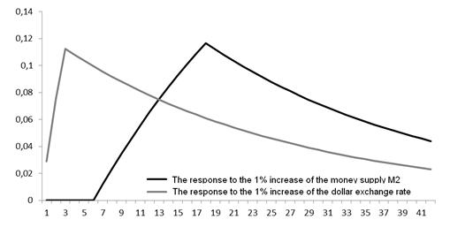
Figure 8. The response of the consumer price index (%) to the growth of the money supply and the dollar rate by 1% to the previous month (the number of the month is on the horizontal axis)

As we can see in Figure 8, the maximum effect of the increase of the growth rate of the money supply and the dollar rate by 1% leads to the growth of the annual consumer price index, approximately by the same value – 0.12% but it is significantly spread out over the time. And, while dollar rate rapidly leapt by dozens percent, which made the contribution of this indicator to the growth of the consumer price index quite significant, the same rapid leaps in the money supply were not observed for the reviewed period. Thereupon, the third hypothesis formulated in the introduction should be described as follows: in the reviewed time period (from 2003 to 2014) the variables of the Bank of Russia’s monetary policy (the money supply and the monetary base) didn’t have any strong effect on the inflation rates.

Therefore, we are able to reach the following conclusion regarding the truth of the 3^rd hypothesis. On the one hand, we cannot recognize the effect of the monetary policy on inflation as an insignificant one, because this link is traced. On the other hand, this effect should never be overestimated.

4. Conclusion

In this article, thanks to the assistance of econometric methods, hypotheses of the effect of monetary policy variables on the Russian economic development indicators were tested. The result of the test is an opportunity to not reject the chances regarding the fact that the variables of the Bank of Russia’s monetary policy (the money supply and the monetary base) have a statistically significant effect on the GDP growth rate and the rouble effective exchange rate. The hypothesis that the variables of the Bank of Russia’s monetary policy (the money supply and the monetary base) have a statistically insignificant effect on the inflation rates was officially rejected. However, it was shown that this effect is rather weak.