Measuring and analyzing the impact of oil price fluctuations on Iraq's gross domestic product (GDP) variable by using the ARDL model for the period (1970–2020)

Introduction

Economies are trying to diversify sources of income, whether developing or advanced, to avoid sudden economic shocks and thus affect the volume of expenditures and revenues and the general economy. On the one hand, and on the other hand, it is noted that there are some countries that have been able to achieve significant developmental leaps, such as the Emirates, Qatar and Kuwait, as this can be deduced from the high levels of income of individuals if compared to the countries of the world and the emergence of industries linked directly or indirectly to the oil sector. It works on the level of productivity and therefore the tendency towards diversifying the economy and getting out of the vicious circle of rentier economies and the problem of increasing dependence on oil revenues, which is the main driver of the economic development process. It is considered a political commodity, and this is what makes dependence on oil a danger to the mentioned economies. The Iraqi economy suffers as a whole Among the concomitant problems, among them are structural and structural imbalances as a result of various factors, including social, legal, political or economic, and a reform process must be taken to lift the economy out of the declining reality at all levels and transform into the ranks of developed countries. It is used as a model and experiment.

There are many studies that dealt with the topic of research, including, Abd al-Rahman Karim Abd al-Ridha al-Tai [1, p. 715-720], The study aims to diagnose the concept of economic growth and the most important factors affecting it and sought to highlight the relationship between oil prices and Iraqi economic growth in the long term and to determine the direction of that effect for the period 1970-2015, and among the most important conclusions, oil will remain the most likely among the alternatives and the oil countries will not be able to compete with the developed countries Unless the rise in oil prices equals the values of imported goods from the above-mentioned countries, so oil maintains its position and considers it a main pillar for the advancement of forward-looking economies.

Chahrazed Madjdoubi ,Aicha Zidelmel Affane , [2, p. 1101-1132],The study tested the impact of fluctuations in the global oil markets on the Algerian economy using the joint integration approach and testing whether there is a long or short-term relationship. It makes the economic situation more difficult, especially in times of crises and global policies, and the study considers it necessary to find new alternatives to rely on in managing the Algerian economy.

Rahim Hassouni Ziyara, Morteza Hadi Janandi Naji [3, p. 430 - 454], The study aimed to analyze the reality of oil wealth in Iraq and the extent of the impact of the oil sector on the rate of inflation and economic growth in Iraq. The study concluded that there is a positive long-term equilibrium relationship between fluctuations in oil prices and GDP, as well as the existence of a causal relationship between crude oil prices and nominal GDP and the absence of that relationship with the inflation rate.

Anthony Msafiri Nyangarika, Alexey Yurievich Mikhaylov, [4, p. 42 - 48], The study sheds light on the degree of correlation between oil prices and GDP for a group of countries, including the Kingdom of Saudi Arabia, as one of the most important suppliers of crude oil to the global market. GDP, as well as the interdependence between the two indicators in the Russian Federation and the Kingdom of Saudi Arabia, and the study emphasized the adoption of alternative sources of energy, through which it is possible to provide opportunities to reform economies and reduce the risk of fluctuations in oil prices.

María Dolores Gadea, Ana Gómez-Loscos, Antonio Montañés, [5, p. 77 - 80], The study deals with research on changes in the relationship between oil prices and the growth rates of the gross domestic product of the American economy according to the long-term perspective, although there are periods in both variables subject of the research, but the lack of influence between the two variables was observed when looking at the period in a comprehensive manner as well as discovering a relationship Partial terms are important, on the one hand, and on the other hand, the study concluded that the impact of the oil price shock causes a decrease in GDP growth over time. As well as a significant negative impact at the time of large increases in oil prices, paralleling the increases.

Results analysis and discussion

The Iraqi economy suffers from the problem of increasing dependence on the rentier resource, which represents the greatest proportion of the recent eras of contribution to the gross domestic product, and therefore this resource has a longitudinal dominance to influence the above variable, the studied time series extends from 1970-2020, the data was extracted from several sources and from international institutions the World Bank and some other local institutions such as the Central Bank of Iraq and the Central Organization for Statistics and Information Technology. The observations were represented in the time series from 1970-2020 as annual observations. This is on the one hand, and on the other hand, the GDP and oil prices represented the variables Studied my agencies:

Table (1) Gross Domestic Product at Oil Prices 1970-2020 (Million Dollars / Dollars)

Looking at the outputs of stability and static, through which one model can be chosen without another, it becomes clear that the variables under study were not all stable at the level, but rather stabilized at the first level and difference and with significant levels of 1% - 5% for the different tests (Dickey Feller Extended Phillips-Peron, Press) and under the assumptions With and without interrupter, with a secant and a direction, and the results were as in the following table:

Table (2) Data stability using unit root (8) for ADF, (PP)

It is necessary to formulate the model to start the process of quantitative analysis to measure the effects of long or short-term relationships by choosing the appropriate model for the nature of (9) study variables and to identify the existing relationships between the variables under study ARDL.

t…….(1)

Since:

Gross domestic product GDP

Constant c

The ability of the dependent variable λ

The first difference in the values of the variable ∆

Estimations of long-term explanatory variables β_1 β_2

Oil prices OILP

slow down for one year t-1

Error limit εt

To delve into the results of the slowed-down gap autoregressive analysis, the results are included in the following table:

figure (1) Akaike information Criterion

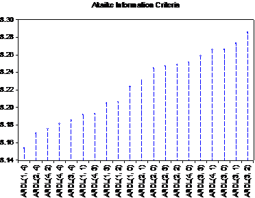
Source: From the researchers’ work based on the results of the statistical program Eviews’ 9.0

The table also shows the different combinations of twenty models, and the lowest value for AIC(10) is model 16, as follows:

Table (5) Lowest Value Test Results for AIC

In a related aspect to the sequence of tests for the aforementioned methodology, we deal with the integration test and the long-term parameters, as the test results showed all significant parameters and the integration equation was as follows

Cointeq = GDP - (5.6817*OILP -123.3321 )

Also, the correction parameter was significant and negative. As for the aspect related to the long-term parameters of the model, the significance of the oil price variable has been proven, and it has a positive relationship to GDP, and the following table supports what was previously interpreted:

Through the limits test (11), it is noted that the test value (9.810637), which is the highest value at all levels, of course, is a good indication of the coherence of the chosen model, as follows:

To complete the tests, it is clear from the following that the residuals are distributed normally with a significant level of 1%, as follows:

figure (2) Jarque – Bera . test

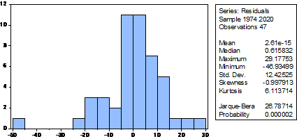
Source: From the researchers’ work based on the results of the statistical program Eviews’ 9.0

In addition to the Breusch-Godfrey Serial Correlation LM test, which shows that the model does not suffer from this problem and related to the mentioned tests, it is clear that the model also does not suffer from the instability of homogeneity of variance depending on the results of the Breusch-Pagan-Godfrey, Glejser and ARCH tests, and as Come:

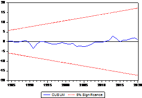
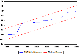
The diagrams of the two tests of the cumulative sum and its squares indicate that the model passed the two mentioned tests and does not suffer from possible structural problems in the future. It can also be noted that the behavior of the phenomenon studied, and to note what we went to interpreting, the following can be seen:

Source: From the researchers’ work based on the results of the statistical program Eviews’ 9.0

figure (4) The cumulative sum square test at 5% significance level

Source: From the researchers’ work based on the results of the statistical program Eviews’ 9.0

Discuss the results

It is clear from the results of the standard aspect analysis that the best combination for the ARDL model is (4, 1), which was chosen from among 20 proposed combinations based on the AIC criterion. (8.153705), which is the lowest value of the combination (16) and the integration equation was GDP – (5>6817*OILP – 123 – 3321) and the results of the analysis showed coherence and significance as in Table (6) for all parameters at the short and long levels, as well as the integration parameter that was Significant and negative at the same time, this is on the one hand, and on the other hand, the speed of adjustment of the model on the equilibrium path amounted to (0.128509), meaning that approximately 12% of the errors can be dealt with during the measurement unit of the model (one year), and the limits test indicates the ability of the chosen model. To explain the relationships in the light of economic theory according to the short and long run, the boundary test value reached (9.810637), which is the highest value of I1 at all levels, which is another indication of the coherence of the model. The dimensionality was considered by God Frey, Pagan, Glejser, ARCH, and the results of the analysis proved that the selected model does not suffer from serial correlation problems for random residuals, as well as the model is free from the problem of instability of homogeneity of variance. Finally, schemes 3 and 4 prove that the model does not suffer from effects Structural changes over time.

In light of the assumptions of the economic theory and when using the ARDL model, it becomes clear that there is a co-integration between oil prices and GDP based on the calculated F-test value, which is greater than the upper boundary value. Joint integration between the two studied variables, the Bound Test table. Table (4) shows that all the variables’ coefficients are in line with the assumptions of the economic theory, as an increase in oil prices by 1% will lead to an increase in the gross domestic product by approximately 6.15%.

Also, the results of the analysis indicate that the null hypothesis is not rejected, as it states that the random errors are normally distributed in the estimated model.

References:

Abd al-Rahman Karim Abd al-Ridha al-Tai (2018). Analysis of the Reality of the Relationship Between International Oil Prices and Economic Growth, Iraq: A Case Study for the Period 1970-2015 Wasit Journal for Human Sciences. (14(1)). 715-762.