Practical aspects of creating an internal rating based model of non-financial companies

Introduction

The letter № 192-Т “On methodical recommendations concerning realisation of the approach to calculating credit risks based on internal ratings of the banks» of The Bank of Russia [2] describes the requirements to credit organisations planning to present their IRB-models for checking on the subject of compliance with Basel II criteria related to implementation of approaches based on internal ratings. Presently, the amount of capital necessary for credit risk cover is calculated according to the instruction № 139-И [3] of The Bank of Russia and other regulatory documents. The approach based on internal ratings is an alternative to the standardized approach to determination of the capital amount necessary for credit risk cover. The standardized approach uses fixed credit risk coefficients within various asset groups recognised by the regulatory body, while IRB-approach enables to determine risk coefficients on the basis of credit organisations’ own systems of internal ratings. RWAs (Risk weighted assets) are calculated on the basis of internal PD assessments (Possibility of Default), LGD assessments (Loss Given Default) and EAD (Exposure at Default) assessments and are used to calculate the required capital minimum value (The Instruction № 139-И). For the transition to IRB-approach a bank needs to have been using this approach in the internal systems of credit risk evaluation and management for, at least, three years (the so-called use test). The amount of the need for capital can be calculated based on IRB-approach if the bank meets minimum criteria, defines the default case according to its regulatory definition, has got historical data for the minimum period (for calculation of PD, LGD and EAD values) etc. The Bank of Russia gives two options as for the IRB-approaches – basic IRB-approach and “advanced” IRB-approach. When using basic IRB-approach, the banks themselves, as a rule, calculate only PD values, while the values of other risk components are calculated by the regulatory authority. Advanced IRB-approach involves self-performed calculations of PD, LGD, EAD and the redemption date terms.

The definition “rating system” includes a set of methods, procedures, control systems, data collection systems and IT-systems that are used to assess credit risks, determine internal ratings of credit claims according to risk level, and to perform quantitative evaluation of the risk of default and losses. A bank has the right to use several rating methods/systems within the frames of each separate class of credit claims. In case bank has several such systems, the decision on referring the lendee to each separate rating system is to be based on internal bank’s documents, according to principles allowing to take into account the credit risks related to each lendee most efficiently. The Bank of Russia describes the minimum requirements to models used in rating systems as follows:

ü The model has to be prognostically reliable. Banks need to compare actual frequency of default cases of the lendees with forecast PD values for each lendee class on a regular basis. It is also necessary to be able to provide documentary evidence that the actual frequency of such defaults remains within the forecast range for the respective lendee class.

ü Model input variables are to be sufficient for obtaining forecast values.

ü The model should not have considerable structural flaws.

An important stage in IRB-approach implementation in a bank is the development of a qualitative model for PD assessment of corporate counterparties that would enable to evaluate their credit quality efficiently enough. The development of such a model is a creative task involving multiple technical details and complexities. In the given article we will discuss difficulties we have encountered during the development of PD assessment model for Russian non-financial sector companies.

A method of creating a PD model

The algorithm for creating the model included the following stages:

1. Identification of the set of potential factors of the model: groups of financial coefficients, macro-indicators; calculation of the selected financial coefficients on the data of the reports;

2. Analysis of the financial coefficients (plotting of ROC-curves, calculation of AUC coefficients (Area Under Curve), selection of indicators having maximum forecasting power, analysis of outliers, discretisation [4]);

3. Testing of different variants of logistic regression model that are evaluated only with use of financial coefficients, choice in favor of the best model variant;

4. Adding of micro-factors to the model determined on stage 3, choice in favour of the best model variant;

5. Appraisal of stability of model coefficients in different periods.

In total, 18 financial coefficients were considered during creation of the PD model. It is possible to divide these coefficients into the following groups:

ü Coefficients of the capital structure and debt burden

ü Profitability coefficients

ü Liquidity coefficients

ü Turnover coefficients

ü Activity range coefficients

The sample used for the analysis and PD model creation contains the data of annual statements (1, 2 forms) of more than 8 000 Russian companies of the non-financial sector for 7 years: about 50 000 observations in total with the share of default observations being on the level of 2,3%. The initial sample was divided into the training and control samples in the ratio of 70%/30% with the requirement that the default levels within each sub-sample be equal [5].

The algorithm application to the data of the sample resulted in creation of the logistic regression model that is presented in Table 1.

Table 1

Logistic regression model coefficients

Financial coefficient	Regression coefficient	Standard error	t-statistics	Probability
Constant	0,2426	0,0929	2,61	<0,001
Profitability of sales	-0,3737	0,0415	-9,01	<0,001
Cash to assets ratio	-13,5979	1,7219	-7,9	<0,001
Operating income to the interests payable ratio	-0,2021	0,0231	-8,7	<0,001
Payables turnover	-0,4114	0,0254	-16,2	<0,001
Capital	-0,2713	0,0216	-12,58	<0,001

Source: compiled by the authors.

Further we will discuss certain aspects and observed empirical facts the authors have encountered when creating the above-presented model.

Analysis of the factors

Dynamic conversions of the factors

In order to select coefficients with the highest forecasting power, not only absolute values of financial coefficients, but also their dynamic conversions have been analysed, namely: growth and absolute gain (in relation to the previous period) rates. Interesting empirical fact: forecasting power of the factors in the sample under consideration decreases in the transition to conversions. Mean change of AUC coefficient in the transition from absolute values to growth rates and absolute gains is about -10%. At that, ROC-curve loses its convexity for most parameters in the transition to conversions, becoming more monotonous. For instance, forecasting power of ROA factor (Return on Assets) in the figure below is, approximately, 1,5 times lower in case of converted factor values.

It should be added that the sample volume considerably decreases in result of transition to dynamic conversions (not all of the reports present in the sample reflect 2 consecutive years), which can have negative impact on the model quality.

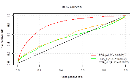
Figure 1. An example of the decrease of the forecasting power of a factor in the transition to dynamic conversions

Source: compiled by the authors.

Discretisation

In case there are outliers in the observations, and in order to enhance the forecasting power of the factors, it is recommended to perform discretisation – the procedure of dividing the whole set of factor values into intervals with assignment of a discrete value to each interval according to particular rules. All factors in the presented model have been discretised by quantile discretisation: the amount of discrete intervals for each variable was chosen on the grounds of the expert evaluation: subject to monotonous change of the share of defaults within intervals.

Consider an example of the forecasting power increase and elimination of ROC-curve non-monotonicity through discretisation: for coefficient Obligations/Capital within the analysed sample, ROC-curve takes the form presented in Figure 2 (to the left); at that, AUC coefficient is 47%. Fig. 3 shows empirical conventional density of the default level from the values of the parameter Obligations / Capital: maximum share of the default observations (almost 10%) is typical of the first (left) interval; from the 2^nd to the 9^th intervals, the share of default observations increases monotonically (from 0,08% to 4,46%). If we arrange the intervals by the share of default observations and assign an ordered discrete value from 1 (for the interval with minimal level of discrete observations) to (for the interval with maximal level of discrete observations) 9 to each interval, this will increase the forecasting power of a factor more than 1,5 times (Figure 2 to the right).

Let us note that discretisation should be performed when there are outliers in the values of financial coefficients or if the ROC-curve of this coefficient is non-monotonic.

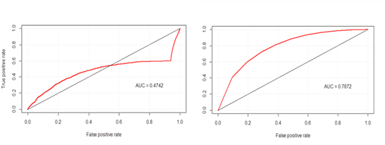
Figure 2. ROC-curve of the parameter Obligations/Capital (to the left – for continuous values, to the right – for discrete ones)

Source: compiled by the authors.

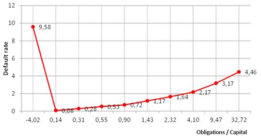
Figure 3. Empirical conventional density of the default rates of the sample, subject to values of the coefficient Obligations / Capital

Source: compiled by the authors.

Use of the macroeconomic variables

After the best model variant with financial coefficients (3^rd stage of the method) has been found, we have tried to improve the forecasting power of this model by adding the following macro-factors [6] (and their conversions) successively:

• GDP (Gross Domestic Product) in main prices;

• M2 to GDP ratio;

• Average official Euro exchange rate;

• Average official USD exchange rate;

• Refinancing rate (as for the 1^st of January of the report year);

• Consumer price index;

• Average oil price (Urals).

In most cases, when a macro-factor was added to the model, the coefficient turned out to be statistically insignificant (statistical significance was determined by t-test). In cases the statistical coefficient was significant, economic interpretation became complicated – the coefficient sign did not make much sense economic-wise (for example, according to the evaluated coefficients it turned out that the higher the inflation was, the lower PD value we had or the higher the refinancing rate was, the lower PD value we had). It is possible that distortion of the influence of macroeconomic factors results from the fact that the sample is unrepresentative as to macroeconomic cycle, i.е. the default level of the sample under analysis in different years does not correspond to the real default level of the economy in these years.

Since financial coefficients implicitly contain the information about the macroeconomic environment, inclusion of macro-factors in the model does not enhance its forecasting power; hence these macro-factors can easily be disregarded in our analysis.

Mapping of the model with an international scale

The final stage of creating a PD assessment model is the determination of the rating scale on the basis of this model. It is often convenient to use an international scale as a benchmark, because its risk classes are mostly comprehensible and easy-to-use for a broad number of experts. We suggest the following algorithm for mapping of a model with an international scale:

См. также:

   Стратегии инвестирования в интеллектуальный капитал под влиянием моделей создания ценности (Деглес Хани С.М., Кельчевская Н.Р.) // Вопросы инновационной экономики. № 4 / 2020

   Методика планирования продовольственной поддержки населения (Самыгин Д.Ю.) // Продовольственная политика и безопасность. № 1 / 2021

1. Rating scale calibration with use of the training scale. A set of risk classes of an international scale is determined. These risks will be included in the IRB-scale (the set of risk classes can be limited from above by the rating of the country whose companies are considered within the sample, for instance). The training sample is ordered in accordance with the descending values of the model. Given the known average default level of each risk class of the international scale, boundary values in the ordered training sample are determined in such a way as to bring the share of defaults in the separated risk classes into compliance with the default level of the respective risk class of the international scale.

2. Testing of the internal scale in the control and full samples. In case of correctly performed calibration of the rating system in the training sample, the default level within various risk classes in the control and full samples will correspond to the default level of risk classes of the international scale.

3. Testing of the scale stability through the creation of migration matrices. Stable and monotonous character of the companies’ default level in the scale of risk classes for annual and mid-annual migration matrices evidences that the model is stable and the risk-scale quality is high.

Let us note also that complete correspondence of the scales is only possible when general default level of the studied sample and the default level of the sample with which the rating agency works coincide. Otherwise, the risk scale under development will be biased with respect to the risk classes of the international scale.

Conclusion

The article provides examples of the method of creating a PD model for the companies of the non-financial sector and also of the method of developing an internal scale of risk classes that would correspond to the international scale. The result of creating such a model for Russian companies has been presented. Following the empirical study results, a number of practical conclusions can be formulated:

1. The forecasting power of the factors can significantly decrease in the transition to dynamic conversions (gains, growth rates);

2. Discretisation of the factor values enables improving their forecasting power and transiting to a monotonous ROC-curve;

3. It is appropriate to include macroeconomic factors in the model in case the sample is representative in relation to the macroeconomic cycle.