The shadow economy and illicit financial flows: evidence of visibility bias in trade-based measurement

1. Introduction

Illicit financial flows (IFFs) are widely regarded as one of the most significant barriers to the financing of sustainable development. According to the 2030 Agenda for Sustainable Development, combating IFFs has been identified as a priority under target 16.4, which calls upon Member States to “significantly reduce illicit financial and arms flows, strengthen the recovery and return of stolen assets and combat all forms of organized crime”. Progress towards this target is monitored through indicator 16.4.1 – namely, the total value of inward and outward IFFs – for which UNCTAD and UNODC have been designated as joint custodian agencies [2] (UNCTAD & UNODC, 2020). However, despite the high level of internationally voiced political commitment, empirical evidence on the structural determinants of IFFs remains comparatively underdeveloped, particularly regarding the role of the shadow economy.

Estimates of the scale of IFFs vary considerably across studies; however, they consistently indicate that trillions of US dollars are transferred annually out of developing economies. According to Global Financial Integrity (GFI), trade misinvoicing alone is estimated to account for at least 500 000 million USD per year in value gaps in developing countries, while money laundering, as estimated by UNODC, is reported to represent between 2 and 5% of global GDP. In many developing economies, such outflows are reported to exceed official development assistance (ODA) inflows, thereby undermining domestic resource mobilisation and widening fiscal gaps. Shadow economy adds a further dimension to this challenge: according to the recent estimates produced by [19] (EY, 2025), 19.3% of global GDP (approximately 20 trillion USD) is reported to operate outside formal oversight. The intersection of these two phenomena is therefore considered to constitute a critical, though under-researched, issue within development economics.

The shadow economy, which is widely understood to encompass unreported income generated through legal production, informal transactions, and outright illegal activity [15] (Schneider et al., 2002), is conceptually intertwined with IFFs. Both phenomena involve economic activity hidden from official oversight; both are reported to erode the tax base and weaken state institutions; and both are shaped by the quality of governance, the regulatory burden, and the enforcement capacity of public authorities. It should also be noted that the UNCTAD/UNODC (2020) Conceptual Framework explicitly locates illicit tax and commercial practices within a broader landscape of shadow economic activity, stating that such flows are “non-observed, hidden or part of the ‘shadow economy’, the underground economy or the informal economy” [2] (UNCTAD & UNODC, 2020, p. 14). Nevertheless, the empirical relationship between the size of the shadow economy and the magnitude of cross-border illicit financial flows has received comparatively little systematic attention to date. Most quantitative studies of IFFs have been focused on methodological refinements, in particular, on the Partner Country Method (PCM), on the Price Filter Method (PFM), and on the piloting of bottom-up estimation frameworks, rather than on the structural determinants that may explain why some economies exhibit larger IFFs than others.

The present paper is intended to address this gap. Specifically, the cross-country association between shadow economy size and the magnitude of detected trade misinvoicing is examined across 111 economies. The central research question is formulated as follows: what is the relationship between the shadow economy and illicit financial flows, as measured through bilateral trade discrepancies? IFFs are operationalised through the PCM applied to mirror statistics from the UN Comtrade database [1], while the shadow economy is measured using the [19] (EY, 2025) enhanced CDA estimates covering 131 economies over the period 2000–2023. The Corruption Perception Index, GDP growth, population, and regional fixed effects are included as control variables.

Considering the theoretical literature, the relationship between the shadow economy and IFFs cannot be stated unambiguously. On one hand, it is suggested that a larger shadow economy may generate a larger volume of illicit cross-border flows, as unreported income is channeled toward foreign safe havens through trade misinvoicing, illicit remittances, or capital flight; under this hypothesis, a positive association would be expected. On the other hand, where the shadow economy is large, it is also suggested that a greater proportion of cross-border value transfer is conducted through informal channels; under this hypothesis, a negative association with detected IFFs would be expected. methods, and to the substitution between formal and informal channels of value transfer.

The analysis presented in this paper yields a paradoxical but informative finding: economies characterized by larger shadow economies are observed to exhibit lower levels of detected trade misinvoicing relative to GDP. It is proposed that this negative association reflects a visibility bias that is inherent in trade-based measurement of IFFs, which is done by application of the PCM method. This method detects discrepancies only within formally recorded customs data, where a substantial share of economic activity occurs through informal channels; such flows remain invisible to mirror trade analysis. Accordingly, the shadow economy coefficient should not be interpreted as reflecting the absence of illicit flows, but rather the proportion of such flows that escapes the formal statistical infrastructure.

The paper makes three contributions. Firstly, a systematic cross-country test of the relationship between shadow economy size and trade-based IFF estimates is presented, with the analysis grounded in the UNCTAD/UNODC Conceptual Framework. Secondly, the robustness of conventional OLS inference is demonstrated by supplementing parametric results with a non-parametric bootstrap test based on 10,000 replications, which addresses sample-size concerns. Finally, an interpretation of the observed relationship is proposed, with direct implications for the design of IFF monitoring frameworks under SDG indicator 16.4.1 and for the complementary role of bottom-up measurement methods in economies with large informal sectors.

The remainder of the paper is structured as follows. In Section 2, the literature on shadow economy estimation, IFF measurement, and the conceptual linkages between the two phenomena is reviewed. In Section 3, the data, the empirical strategy, and the diagnostic framework are described. In Section 4, the main results and the corresponding robustness checks are presented. In Section 5, the findings, their implications, and their limitations are discussed. In Section 6, the conclusions are summarized.

2. Literature review

2.1. Conceptual framework

According to the UNCTAD/UNODC Conceptual Framework for the Statistical Measurement of Illicit Financial Flows [2] (UNCTAD & UNODC, 2020), IFFs are defined as “financial flows that are illicit in origin, transfer or use, that reflect an exchange of value and that cross-country borders”. Within the framework, four categories of IFF-generating activities are identified: (1) illicit tax and commercial practices (including both illegal tax evasion and aggressive tax avoidance through base erosion and profit shifting); (2) illegal markets; (3) corruption (including bribery, embezzlement, and illicit enrichment, as defined under the UN Convention against Corruption); and (4) exploitation-type activities and the financing of terrorism. Within each category, IFFs are reported to emerge at two stages: income generation and income management.

The shadow economy, which is understood to encompass unreported legal production, informal transactions, and illegal activity [15, 17] (Schneider et al., 2002; Schneider et al., 2017), is reported to overlap substantially with the first IFF category. As noted in the said Framework, illicit tax and commercial IFFs correspond to activities that are “non-observed, hidden or part of the ‘shadow economy’, the underground economy or the informal economy”. Accordingly, the central empirical question addressed in this study is formulated as follows: whether larger shadow economies are associated with higher or with lower levels of detected IFFs.

2.2. Shadow economy estimation

It should be noted that no universally recognized method for the estimation of the shadow economy currently exists. Earlier in the articles, we tested various methods for calculating the scale of the shadow economy [9, 10] (Maga, 2020; Maga et al., 2019). We also reviewed the methodological foundations for measuring the scale of the shadow economy [22] (Burov et al., 2022). Direct methods are reported to collect information from market participants through interviews, expert evaluations, and surveys [5, 11, 13] (Frey et al., 1982; Noelle-Neumann, 1974; OECD, 2017). The mentioned methods are widely criticized on the grounds that they are imprecise and subject to response bias [18] (Schneider et al., 2013); nevertheless, they are valued for their capacity to address the exact variables of interest [21] (Williams et al., 2013). Indirect methods are reported to use secondary data – including income-expenditure discrepancies, electricity consumption, monetary aggregates, and latent-variable models – to detect unobserved shadow activity.

For the purposes of this study, shadow economy estimates have been drawn from the EY (2025) Shadow Economy Exposed report, through which estimates are provided for 131 economies over the period 2000–2023 by means of an enhanced Currency Demand Approach (CDA). Under the CDA, the demand for currency is econometrically decomposed into formal and shadow components, with Bayesian model averaging (BMA) being employed for variable selection [4] (Dybka et al., 2019). A distinction is drawn between “committed” and “passive” shadow activity. According to EY estimates, the global average shadow economy stood at 19.3% of GDP in 2023, with 119 of 131 economies reporting declines since 2000. It is reported that the CDA offers advantages over alternative approaches (MIMIC, D(S)GE models), in that both the level and the dynamics of the shadow economy may be estimated using publicly available data [18, 19] (Schneider al., 2013; EY, 2025).

2.3. IFF measurement: The Partner Country Method (PCM)

Among the various measurement approaches developed, the PCM is reported to be the most widely used for trade-related IFFs [2, 6] (UNCTAD & UNODC, 2020; Gara et al., 2019). Under the PCM, the reported export value from country A to country B is compared with the reported import value by country B from country A, with an adjustment for the CIF/FOB margin (typically estimated at 6%). Persistent discrepancies that cannot be explained by known asymmetries may indicate trade misinvoicing. The PCM has been applied by GFI, UNCTAD, UNESCAP, and by national statistical offices.

However, the PCM is reported to suffer from well-documented limitations, in particular, sensitivity to non-IFF asymmetries arising from re-exports (i.e., “grey re-export” and “false transit” arrangements), timing lags, classification differences, and confidential trade flows [12] (Nyasulu et al., 2023). Nevertheless, the PCM is reported to remain the most feasible method for producing comparable cross-country estimates, particularly in developing economies where alternative data sources are limited or unavailable.

2.4. Policy context

According to Schneider [14] (Schneider, 2015), indirect taxes, self-employment, and unemployment are identified as the principal drivers of the shadow economy. Significant links between the shadow economy and institutional quality [3, 16] (Dreher et al., 2010; Torgler et al., 2007), globalization [1] (Berdiev et al., 2018), and foreign direct investment [8] (Huynh et al., 2020) have been documented in the literature. Within the EY (2025) report, a distinction is drawn between policies targeting “committed?” activity (i.e., enforcement, formalization incentives, and tax-morale measures) and those addressing “passive” concealment (i.e., digital payments and electronic receipts). The policy dimension is reported to be directly relevant to IFFs: reduction of the shadow economy through institutional strengthening should be expected to curtail cross-border illicit flows, whilst IFF countermeasures, including customs data sharing, beneficial ownership transparency, and the automatic exchange of tax information (AEOI), may be expected to reduce the domestic shadow economy by raising the cost of concealment. Data sharing arrangements, such as customs unions (EAEU, EU/EEA, ASEAN, MERCOSUR) and bilateral Trade Transparency Units (TTUs), are reported to have potential effects on misinvoicing detection.

3. Data and methodology

3.1. Data sources and sample construction

The analysis presented in this paper is based upon a merged panel dataset of 225 country-year observations covering 116 economies in the reference years 2019 and 2023. The dataset has been constructed from six primary data sources. Estimates of illicit financial flows (IFFs) have been derived from the Partner Country Method (PCM) applied to bilateral trade data drawn from the UN Comtrade database for the reference years 2019 and 2023, in line with the methodology endorsed by the UNCTAD/UNODC Conceptual Framework (UNCTAD & UNODC, 2020). Total IFFs are computed as the sum of inward IFFs (i.e., import over-invoicing and export over-invoicing) and outward IFFs (i.e., import under-invoicing and export under-invoicing) at the country level, with an adjustment for a standard 6% CIF/FOB margin applied to imports (GFI, 2019). Shadow economy estimates have been drawn from the EY (2025) enhanced Currency Demand Approach (CDA) covering 131 economies over the period 2000–2023; values for 2019 and 2023 have been used directly. The variable set is completed through the Corruption Perceptions Index (CPI) of Transparency International, the GDP, population and consumer price inflationdata from the World Development Indicators (WDI) of the World Bank.

Of the 116 economies covered, 109 are observed at both reference years, while seven are observed at only one of the two years; the resulting unbalanced panel contains 116 observations for 2019 and 109 observations for 2023, for a total of 225 country-year observations. A binary year dummy (year 2023) has been included in all specifications, by which the common 2019–2023 macroeconomic shock (i.e., the post-pandemic recovery and the subsequent inflationary period) is absorbed. Since the Corruption Perceptions Index covers only the period from 2020 onwards, the 2020 CPI values have been used for the 2019 observations as a one-year-lag proxy; this treatment is supported by the fact that year-on-year changes in the CPI are reported to be minimal. Regional fixed effects have been included to absorb unobserved continent-level heterogeneity. Descriptive statistics for the panel are reported in Table 1.

Table 1

Descriptive statistics for the pooled panel (N = 225)

Variable	N	Mean	SD	Min	Median	Max
IFFs (% of GDP)	225	186.83	189.67	18.16	134.67	923.88
IFFs per capita (USD)	225	41 242	60 878	395	14 796	380 557
Shadow economy (% GDP)	225	18.77	12.67	2.10	17.40	56.30
Corruption CPI	225	47.28	18.42	17.00	42.00	90.00
CPI inflation (%)	225	7.01	17.89	-1.93	3.65	221.34
GDP growth (%)	225	2.92	4.13	-15.33	2.58	33.80
log(Population)	225	16.43	1.58	12.83	16.26	21.09
log(GDP per capita)	225	9.12	1.46	5.38	9.21	11.80

3.2. Variable construction and transformation

The dependent variable is log(IFFs/GDP), where IFFs are reported as a percentage of GDP. The logarithmic transformation has been applied in order to address the right-skewness observed within the raw IFF distribution; thus, an approximately normally distributed dependent variable is obtained. As a robustness check, an alternative specification employing log(IFFs per capita) as the dependent variable has been estimated (Model 6).

It should be noted that the structural predictors – namely, the shadow economy (% of GDP), corruption (CPI), and log GDP per capita – are highly intercorrelated within the panel. The correlation between the shadow economy and log GDP per capita stands at r = -0.93, whilst that between corruption and GDP per capita is reported as r = +0.82. The multicollinearity patterns do not allow simultaneous inclusion of all three development proxies. Therefore, the empirical strategy has been organised into the following stages:

(a) separate models in which each proxy is entered alone (Models 1–3);

(b) a joint specification, in which the shadow economy and corruption are entered together (Model 4, preferred);

(c) a full specification, in which all three proxies are entered simultaneously (Model 5, sensitivity check);

(d) an alternative dependent variable specification, in which log(IFFs per capita) is employed (Model 6). The macroeconomic controls (CPI inflation and GDP growth), log population, the year dummy, and regional dummies are included in all specifications.

The preferred specification (Model 4) is expressed as follows. Let yᵢₜ denote the log-transformed IFFs/GDP ratio for country i in year t (where t ∈ {2019, 2023}); SEᵢₜ the shadow economy share of GDP; CPIᵢₜ the Corruption Perceptions Index (in which higher scores indicate less corruption); D2023ₜ the year dummy equal to (1) for year 2023 and 0 otherwise; and Xᵢₜ a vector of macroeconomic controls (i.e., CPI inflation, GDP growth, and log population) together with regional dummies. The said model is specified as:

yᵢₜ = α + β₁ SEᵢₜ + β₂ CPIᵢₜ + τ D2023ₜ + γ′ Xᵢₜ + εᵢₜ, (1)

where εᵢₜ is the error term, which is assumed to be independent across countries but is permitted to be correlated within countries across the two reference years. The coefficients β₁ and β₂ are considered to be the parameters of primary interest.

A negative coefficient on the shadow economy (i.e., β₁ < 0) would indicate that economies characterized by larger shadow economies exhibit lower levels of detected trade misinvoicing relative to GDP, ceteris paribus. A negative coefficient on the CPI (i.e., β₂ < 0), given that higher CPI scores indicate less corruption, would imply that more corrupt economies (i.e., those with lower CPI scores) exhibit higher levels of detected IFFs. The sign of β₁ is considered to constitute the central empirical question of the present study.

3.3. Estimation and inference

All models have been estimated by pooled ordinary least squares (OLS) on the panel of 225 country-year observations. All parametric results have been further supplemented by non-parametric cluster bootstrap inference (B = 10,000 replications), by which countries (rather than individual observations) are resampled as units, with their two-year observations kept together. The bootstrap methodology and corresponding full results are reported in Appendix B.

Model diagnostics include the Breusch–Pagan test for heteroskedasticity, the Jarque-Bera test for residual normality, the Durbin–Watson statistic for autocorrelation, and the variance inflation factors (VIFs) for multicollinearity. The results are reported in Appendix A, alongside graphical diagnostics (i.e., residual plots, Q–Q plots, residual histograms, and coefficient forest plots).

The estimation procedure may be summarized as follows:

- Step 1. The PCM is applied to bilateral trade flows from UN Comtrade for the reference years 2019 and 2023, with the CIF/FOB adjustment of 6% applied to import values, in accordance with GFI recommendation.

- Step 2. Inward and outward IFFs are aggregated at the country-year level, and the dependent variable IFFs/GDP is computed; the logarithmic transformation is then applied.

- Step 3. The panel dataset is merged with the EY (2025) shadow economy estimates, the CPI from Transparency International, and the macroeconomic controls drawn from the World Bank and IMF, by which a panel of 225 country-year observations is obtained; the 2020 CPI values are used as a one-year-lag proxy for the 2019 observations.

- Step 4. Six pooled OLS specifications are estimated, ranging from single-predictor models to the full collinear model; in all specifications, a year dummy and regional fixed effects are included, and cluster-robust standard errors (clustered by country) are reported.

- Step 5. Diagnostic tests are performed (see Appendix A), and non-parametric cluster bootstrap inference (B = 10,000) is applied to the preferred specification (see Appendix B), with countries resampled as units.

- Step 6. A preferred specification (Model 4) is identified, in which both the shadow economy and corruption are entered jointly; both coefficients are reported to be statistically significant under cluster-robust inference (p ≤ 0.01), and both effects are confirmed under the cluster bootstrap (p ≤ 0.02).

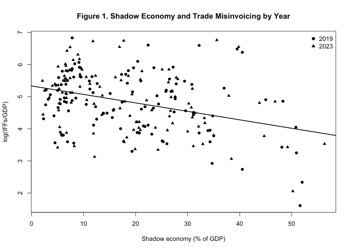
Figure 1. Shadow economy and trade misinvoicing (log IFFs/GDP, panel N = 225)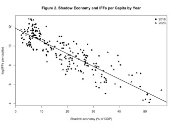

Figure 2. Shadow economy and IFFs per capita (panel N = 225)

4. Results

4.1. Main regression results

In Table 2, six specifications estimated on the panel of 225 country-year observations are reported. In Models 1–3, each structural predictor has been entered individually alongside the macroeconomic controls, the year dummy, and the regional fixed effects. The shadow economy enters significantly when entered alone (Model 1: β = -0.015; p = 0.092), whereas corruption (Model 2) and log GDP per capita (Model 3) are not individually significant under cluster-robust inference. The said three models yield adjusted R² values in the range of 0.26-0.28. In all specifications, log population is reported to be a significant predictor (β ≈ -0.10 to -0.13; p < 0.05), by which it is indicated that smaller economies exhibit higher IFFs relative to GDP. The year dummy is reported to be positive and statistically significant in several specifications (e.g., Model 2: β = +0.101; p = 0.040), by which a modest rise in detected misinvoicing between 2019 and 2023 is indicated.

Table 2

Pooled panel OLS regression results (N = 225, cluster-robust SEs)

	(1)	(2)	(3)	(4)	(5)	(6)
DV:	log(IFF/GDP)	log(IFF/GDP)	log(IFF/GDP)	log(IFF/GDP)	log(IFF/GDP)	log(IFF/cap)
Shadow economy	-0.015*			-0.032***	-0.048**	-0.116***
	(0.009)			(0.011)	(0.019)	(0.008)
Corruption		-0.004		-0.015***	-0.010
		(0.004)		(0.006)	(0.007)
log(GDP/cap)			+0.033		-0.220
			(0.074)		(0.191)
CPI inflation	-0.003*	-0.005**	-0.004*	-0.005**	-0.005***	-0.007***
	(0.002)	(0.002)	(0.002)	(0.002)	(0.002)	(0.002)
GDP growth	+0.002	-0.013	-0.007	+0.000	-0.002	-0.007
	(0.030)	(0.035)	(0.034)	(0.029)	(0.031)	(0.036)
log(Pop.)	-0.099**	-0.129***	-0.120***	-0.089**	-0.085**
	(0.043)	(0.041)	(0.042)	(0.042)	(0.041)
Year 2023	+0.071*	+0.101**	+0.087*	+0.066	+0.096*	+0.196***
	(0.043)	(0.049)	(0.048)	(0.043)	(0.053)	(0.047)
R²	0.310	0.294	0.292	0.344	0.352	0.815
Adj. R²	0.281	0.264	0.262	0.313	0.319	0.808
N	225	225	225	225	225	225
Clusters	116	116	116	116	116	116

Notes: * p < 0.10; ** p < 0.05; *** p < 0.01. Region dummies included (not shown).

In Model 4 (preferred), the shadow economy and corruption have been entered jointly. The shadow economy coefficient is reported as -0.0316 (cluster-robust p = 0.005), and corruption as -0.0148 (cluster-robust p = 0.009). The adjusted R² is reported as 0.313; furthermore, all variance inflation factors (VIFs) are reported to remain below 3.6, by which acceptable multicollinearity is indicated. The macroeconomic controls CPI_inflation (β = -0.0047; p = 0.012) and log population (β = -0.089; p = 0.034) are also reported to enter significantly. The year dummy in Model 4 is reported as +0.066 (p = 0.125), by which it is suggested that, once the structural predictors are controlled for, the 2019–2023 shift in detected misinvoicing is largely absorbed.

In Model 5, log GDP per capita is added as a further control. The shadow economy coefficient is reported to strengthen to -0.0475 (cluster-robust p = 0.011); however, both corruption (p = 0.128) and log GDP per capita (p = 0.250) lose significance, owing to the severe multicollinearity (the correlation between the shadow economy and log GDP per capita is r = -0.93). The said specification has been reported for the sake of completeness as a sensitivity check, although it is not preferred. In Model 6, log IFFs per capita is employed as the dependent variable, and population and corruption are omitted (since population enters mechanically into the normalization and corruption is replaced by the implicit development gradient). The shadow economy coefficient is reported as -0.1157 (cluster-robust p < 0.001), with an adjusted R² of 0.808; by this finding, it is suggested that the per-capita normalization captures substantially more cross-country variation in trade integration than the GDP normalization does.

4.2. Diagnostic summary

The Breusch-Pagan test indicates the presence of heteroskedasticity in both preferred models (Model 4: χ² = 32.60; p < 0.001; Model 6: χ² = 29.97; p < 0.001). This is consistent with the cross-country nature of the panel, in which economies of widely differing sizes and trade structures are observed, and is the principal reason why cluster-robust standard errors (which are robust to arbitrary heteroskedasticity within clusters) have been used throughout the analysis. The Jarque-Bera test for residual normality is not rejected in either model (Model 4: p = 0.070; Model 6: p = 0.624). The Durbin-Watson statistics are reported as 1.19 for Model 4 and 1.22 for Model 6; these values indicate the presence of positive within-cluster correlation between the 2019 and 2023 observations for the same country, which is precisely the dependence that the cluster-robust standard errors accommodate. All variance inflation factors in Model 4 are reported to remain below 3.6, with the shadow economy variable at 3.58 and corruption at 2.48; for Model 6, the maximum VIF is 3.11. Full diagnostic tables are reported in Appendix A.

4.3. Bootstrap robustness

The non-parametric cluster bootstrap (B = 10,000, with countries resampled as units) confirms the parametric findings under a non-parametric inference (full results in Appendix B). The shadow economy coefficient is reported to be significant at the 5% level (bootstrap p = 0.015), with a 95% percentile confidence interval of [-0.052; -0.006] that excludes zero. Corruption is reported to be significant at the same level (bootstrap p = 0.015), with a 95% percentile confidence interval of [-0.025; -0.003]. The two effects are reported to be of comparable robustness. The population effect is borderline (bootstrap p = 0.053), reflecting some sensitivity to the influence of small island economies in the sample. The bootstrap mean R² is reported as 0.388 (full sample: 0.344), with a 95% confidence interval of [0.262; 0.524], indicating a stable model fit.

5. Discussion

5.1. Interpreting the visibility bias

The negative shadow economy coefficient warrants careful interpretation. It has been observed that economies characterized by larger shadow economies exhibit lower levels of detected trade misinvoicing relative to GDP. Three ways are proposed by which this seemingly paradoxical finding may be explained.

Firstly, it should be noted that the PCM is capable of detecting discrepancies only within recorded trade. Where cross-border economic activity is conducted through informal channels, such as smuggling, informal value transfer systems (e.g., hawala networks), unreported remittances, or barter-based trade, such flows are not recorded in customs data and therefore remain invisible to mirror trade analysis. Accordingly, the shadow economy variable serves as a proxy for the share of total economic activity that escapes the formal statistical infrastructure upon which the PCM depends. In economies in which the said share is large, the denominator of unmeasured illicit flows is reported to grow relative to the numerator of measured trade discrepancies.

Secondly, economies characterized by large shadow economies are reported to be less formally integrated in official trade channels. Their formal trade volumes are reported to be lower relative to total economic activity, by which the IFFs/GDP ratio is mechanically reduced, even where misinvoicing rates within recorded trade are reported to be comparable. The shadow economy coefficient is therefore considered to capture not only the direct substitution of informal for formal channels, but also the indirect effect of lower formal trade openness.

Thirdly, it should be noted that trade misinvoicing is primarily a technique employed by formal-sector firms with access to international banking and transparent customs documentation. In economies where the formal sector is relatively small, fewer firms are considered to have the institutional capacity to engage in sophisticated misinvoicing schemes. The absolute volume of detectable misinvoicing may therefore be lower, even where the total volume of cross-border illicit value transfer (i.e., through both formal and informal channels) is reported to be higher.

Considering the three channels described above, a single methodological implication is reached: the PCM is capable of capturing only the visible component of IFFs. The shadow economy coefficient is therefore understood to measure the size of the so-called visibility bias. Important consequences for SDG 16.4.1 monitoring follow from this conclusion: economies with large shadow economies may appear to exhibit lower IFFs when, in fact, a substantial share of illicit flows is simply undetectable by trade-based methods.

5.2. The role of corruption

Corruption is reported to enter significantly in the preferred model under both cluster-robust inference (cluster-robust p = 0.009) and the cluster bootstrap (bootstrap p = 0.015); weaker governance is reported to be associated with higher detected IFFs. The said finding is consistent with the institutional-quality literature [3, 16] (Dreher et al., 2010; Torgler et al., 2007) and with the UNCTAD/UNODC Framework’s identification of corruption as both a generator and an enabler of IFFs. In economies in which anti-corruption institutions are reported to be weaker, misinvoicing may be facilitated through inadequate customs scrutiny, through collusion between traders and officials, and through ineffective enforcement of trade documentation requirements. The fact that corruption retains significance after controlling for the shadow economy suggests that institutional quality is operating through a distinct channel: namely, the shaping of the enabling environment for formal-sector misinvoicing, rather than the relative size of formal versus informal economic activity.

5.3. Population and regional effects

Population is reported to constitute the strongest predictor across all specifications, with smaller economies exhibiting higher IFFs/GDP ratios. The said finding is considered to be a mechanical artefact of trade openness scaling: smaller economies are reported to have higher trade-to-GDP ratios, by which the IFF/GDP numerator is amplified. The Europe dummy is reported to be consistently positive and significant; thus, it is indicated that European countries exhibit higher detected misinvoicing relative to Africa, after the development proxies have been controlled for a finding which may potentially reflect Europe’s deep integration into global supply chains and the higher granularity of European trade documentation. Oceania is reported to exhibit the most negative regional effect; this finding is considered to be consistent with the comparatively simpler trade structures and smaller number of trading partners that are characteristic of island economies.

5.4. Implications for SDG 16.4.1 monitoring

The findings reported herein are considered to have direct implications for the ongoing international effort to monitor progress towards SDG target 16.4. According to the UNCTAD/UNODC Conceptual Framework, a bottom-up, activity-based approach to the measurement of IFFs is recommended, with separate estimation undertaken for different IFF types. The present results are reported to provide empirical support for the said recommendation, in that it is demonstrated that top-down, trade-based estimates systematically underrepresent IFFs in economies characterized by large shadow economies. For custodian agencies responsible for the compilation of national and global IFF estimates, it is implied that PCM-based figures should be interpreted as floor estimates rather than as comprehensive measures – particularly for economies located in Sub-Saharan Africa, South Asia, and Central Asia, where shadow economies are reported to be the largest.

Moreover, the visibility bias is reported to have implications for the interpretation of cross-country IFF rankings. Economies that appear to exhibit lower IFFs in PCM-based analyses may not, in fact, be characterized by lower levels of illicit activity; rather, a larger share of their illicit activity may be conducted outside formal trade channels. Therefore, it is suggested that composite indicators combining trade-based estimates with other approaches – such as balance-of-payments residuals, offshore wealth estimates, and financial intelligence data – would provide a more accurate picture of the overall IFF burden.

5.5. Limitations

Several limitations should be acknowledged. Firstly, it should be noted that PCM-based IFF estimates capture gross bilateral discrepancies, which include non-IFF asymmetries (i.e., re-exports, classification differences, and timing lags). The resulting IFF estimates should therefore be interpreted as upper-bound indicators rather than as precise measurements. Secondly, the pooled panel design (with only two reference years and 92–99% of the variation between rather than within countries) precludes causal identification through fixed-effects techniques; the negative shadow economy coefficient should therefore be considered an association rather than a causal effect. Thirdly, the shadow economy estimates drawn from the EY Currency Demand Approach carry their own measurement uncertainty, which is not propagated into the regression standard errors. Fourthly, the use of the 2020 CPI values as a one-year-lag proxy for the 2019 observations introduces a minor measurement consideration, although year-on-year changes in the CPI are reported to be small and unlikely to materially affect the coefficient estimates. Fifthly, the panel of 225 country-year observations excludes those economies without adequate data coverage; thus, the risk of selection bias cannot be ruled out. The analysis should be repeated with higher data coverage.

6. Conclusion

In the present paper, the cross-country relationship between the shadow economy and illicit financial flows, as measured through bilateral trade discrepancies, has been examined across a panel of 225 country-year observations covering 116 economies in the reference years 2019 and 2023. The central finding is reported as follows: economies characterized by larger shadow economies exhibit lower levels of detected trade misinvoicing – a result which is interpreted as a “visibility bias” inherent in trade-based measurement. The PCM is reported to capture only the portion of illicit value transfer conducted through formal customs channels; where informal economic activity is extensive, the unmeasured share of IFFs is correspondingly larger. Furthermore, corruption is reported to independently predict higher detected IFFs, by which the institutional-quality channel emphasized within the UNCTAD/UNODC Conceptual Framework is confirmed.

Three policy implications appear. Firstly, it is recommended that IFF monitoring under SDG indicator 16.4.1 should not rely exclusively upon trade-based methods: economies with large shadow economies may appear to exhibit lower IFFs when, in fact, a substantial share of illicit flows is simply invisible to mirror trade analysis. Therefore, it is advised that national statistical offices (NSOs) and international custodian agencies should interpret PCM-based estimates in light of the shadow economy context. Secondly, capacity-building efforts should be prioritized toward the development of complementary measurement approaches – in particular, bottom-up methods for illegal markets, financial intelligence analysis, and transaction-level customs data analysis through the Price Filter Method (PFM), to avoid visibility bias. Thirdly, anti-corruption measures are considered to remain independently important: even after the shadow economy has been controlled for, governance quality is reported to constitute a significant predictor of misinvoicing, by which the need for integrated policy responses (addressing both institutional weakness and the formalization of economic activity) is confirmed.

It is recommended that future research should extend the present analysis along several dimensions: longer time panels, by which within-country identification may be enabled as shadow economies evolve over time; integration of other IFF proxies; the incorporation of data-sharing agreement controls, by which it may be tested whether customs transparency mechanisms moderate the shadow economy-IFF relationship; and an addition of qualitative assessment through country case studies, by which the specific mechanisms through which informal economic activity generates invisible cross-border financial flows may be traced.

Appendix A. Diagnostic tests and model assumptions

Homoskedasticity. Under the Breusch-Pagan test, the squared OLS residuals are regressed upon the fitted values, with a view to the detection of systematic heteroskedasticity. For Model 4, the test statistic is reported as 32.60 (p < 0.001); for Model 6, χ² = 29.97 (p < 0.001). Both tests reject the null hypothesis of constant error variance at conventional levels – a finding which is consistent with the cross-country nature of the panel, in which economies of widely differing trade volumes and institutional contexts are observed. The cluster-robust standard errors (which are robust to arbitrary heteroskedasticity within clusters) employed in the main estimation, and the cluster bootstrap, provide robust inference notwithstanding the said heteroskedasticity.

Normality. The Jarque–Bera test for Model 4 yields JB = 5.31 (p = 0.070); for Model 6, JB = 0.94 (p = 0.624). In neither case is the null hypothesis of normally distributed residuals rejected at the 5% level. The residual histogram (Figure A3) and the Q–Q plot (Figure A2) are reported to confirm approximately normal residuals with slight positive skewness for Model 4.

Autocorrelation. The Durbin–Watson statistic is reported as 1.19 for Model 4 and 1.22 for Model 6. The said values, which lie below the ideal value of 2.0, reflect positive within-country correlation between the 2019 and 2023 observations.

Multicollinearity. The variance inflation factors (VIFs) for Model 4 are reported in Table A2. The maximum VIF is reported as 3.58 (shadow economy), which is well below the conventional thresholds of 5 or 10. Corruption exhibits a VIF of 2.48. The macroeconomic controls, the year dummy, and the regional dummies are reported to display VIFs below 3.2.

Table A1

Specification and diagnostic tests (panel, N = 225)

Test	Model 4	Model 6
Breusch–Pagan stat	32.602	29.968
BP p-value	<0.001	<0.001
Jarque–Bera stat	5.313	0.944
JB p-value	0.070	0.624
Durbin–Watson	1.193	1.221
Max VIF	3.577	3.112
R²	0.344	0.815
Adj. R²	0.313	0.808
Observations (country-year)	225	225
Clusters (countries)	116	116

Table A2

Variance inflation factors (panel, N = 225)

Variable	Model 4	Model 6
Shadow economy	3.577	2.006
Corruption CPI	2.482	-
CPI inflation	1.121	1.097
GDP growth	1.140	1.122
log(Population)	1.216	-
Year 2023 dummy	1.060	1.059
Americas	1.982	1.895
Asia	2.500	2.296
Europe	3.113	3.112
Oceania	1.216	1.202

In Figure A1, the residuals are plotted against the fitted values for Model 4. The scatter exhibits no clear systematic pattern in the level of residuals, although some funneling consistent with the detected heteroskedasticity is observable. Outliers (|residual| > 1.5) are labeled within the figure; the said outliers comprise both observation years and predominantly represent persistent country-level deviations rather than year-specific shocks.

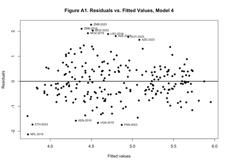
Figure A1. Residuals vs. fitted values (Model 4, panel)

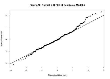
Figure A2. Normal Q–Q plot of residuals (Model 4, panel)

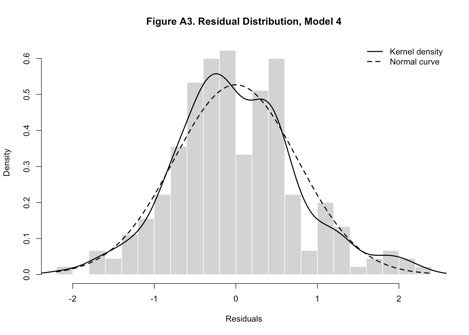
Figure A3. Residual distribution (Model 4, panel)

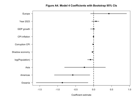
Figure A4. Coefficient estimates with cluster bootstrap 95% confidence intervals (Model 4, panel)

Appendix B. Cluster bootstrap inference

B.1. Rationale

The estimation sample comprises 225 country-year observations covering 116 economies for the reference years 2019 and 2023. Although cluster-robust standard errors (clustered by country) have been employed throughout the main estimation, which may be sensitive to the influence of a small number of outlying countries, the heavy-tailed nature of cross-country trade volume distributions, and the unbalanced structure of the panel (seven economies are observed at only one of the two reference years). For these reasons, the parametric results have been supplemented with non-parametric cluster bootstrap inference, which constructs the empirical sampling distribution of each coefficient directly from the data, without distributional assumptions and with explicit respect for the dataset's panel structure.

B.2. Procedure

The bootstrap procedure may be summarized as follows:

Step 1. In each of B = 10,000 replications, a sample of 116 countries is drawn with replacement from the original panel; for each sampled country, all available observations are retained.

Step 2. The full pooled OLS model (Model 4) is re-estimated on the bootstrap sample.

Step 3. The bootstrap standard error is computed as the standard deviation of the 10,000 coefficient estimates.

Step 4. The 95% confidence interval is computed as the 2.5^th–97.5^th percentile interval of the bootstrap distribution.

Step 5. The bootstrap p-value is computed.

B.3. Results

Table B1

Cluster bootstrap inference for Model 4 (B = 10,000, panel N = 225)

Variable	Point	Boot SE	Boot Mean	95% Low	95% High	p (boot)
Shadow economy	-0.0316	0.0117	-0.0298	-0.0518	-0.0058	0.015
Corruption	-0.0148	0.0058	-0.0140	-0.0252	-0.0026	0.015
CPI infl.	-0.0047	0.0056	-0.0040	-0.0121	+0.0123	0.196
GDP growth	+0.0003	0.0347	-0.0110	-0.0893	+0.0360	1.000
log(Pop.)	-0.0887	0.0432	-0.0870	-0.1691	+0.0010	0.053
Year 2023	+0.0657	0.0488	+0.0577	-0.0448	+0.1485	0.225
Americas	-0.5797	0.2489	-0.5923	-1.0892	-0.1142	0.015
Asia	-0.2571	0.2890	-0.2381	-0.8159	+0.3171	0.417
Europe	+0.4254	0.2519	+0.4307	-0.0682	+0.9160	0.093
Oceania	-0.8705	0.4071	-0.8304	-1.6126	+0.0000	0.108
Constant	+7.6460	0.8261	+7.5808	+5.9665	+9.2360	<0.001

Notes: Cluster bootstrap with countries resampled as units (B = 10,000). 95% CI = percentile interval. R² point: 0.344; boot mean: 0.388; 95% CI: [0.262; 0.524].

In Table B1, the full cluster bootstrap results are reported. The bootstrap is reported to confirm the parametric findings under a fully non-parametric inference framework. The shadow economy coefficient is reported to be significant at the 5% level (bootstrap p = 0.015), with a percentile confidence interval of [-0.0518; -0.0058] that excludes zero. Corruption is similarly significant (bootstrap p = 0.015), with a percentile confidence interval of [-0.0252; -0.0026]. The population effect is borderline (bootstrap p = 0.053), with a CI of [-0.1691; +0.0010]. CPI inflation is no longer significant under the bootstrap. The bootstrap mean R² is 0.388, with a 95% confidence interval of [0.262; 0.524], by which a stable model fit is indicated. The bootstrap coefficient distributions for the shadow economy and corruption variables are displayed in Figure B1.

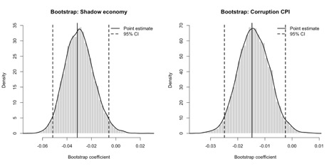
Figure B1. Cluster bootstrap distributions of key coefficients (B = 10,000, panel)

[1] https://comtrade.un.org.

References:

Illicit financial flows to and from 148 developing countries: 2006-2015 (2019). Washington, DC: Global Financial Integrity.
Berdiev A.N., Saunoris J.W. (2018). Does globalization affect the shadow economy? The World Economy. 41 (1). 222-241. doi: 10.1111/twec.12549.
Burov V.Yu., Tumunbayarova Zh.B., Khanchuk N.N., Masalov P.V. (2022). Issues of countering the shadow economy in the scientific literature. Vestnik of Saint Petersburg University. 38 (3). 462-494. doi: 10.21638/spbu05.2022.306.
Conceptual framework for the statistical measurement of illicit financial flowsUnctad.org. Retrieved from https://unctad.org/publication/conceptual-framework-statistical-measurement-illicit-financial-flows
Dreher A., Schneider F. (2010). Corruption and the shadow economy: an empirical analysis Public Choice. 144 (1). 215-238. doi: 10.1007/s11127-009-9513-0.
Dybka P., Kowalczuk M., Olesiński B., Torój A., Rozkrut M. (2019). Currency demand and MIMIC models: towards a structured hybrid method of measuring the shadow economy International Tax and Public Finance. 26 (1). 4-40. doi: 10.1007/s10797-018-9504-5.
Frey B.S., Weck H., Pommerehne W.W. (1982). Has the shadow economy grown in Germany? An exploratory study Review of World Economics. 118 (2). 499-524. doi: 10.1007/BF02706263.
Gara M., Giammatteo M., Tosti E. Magic mirror in my hand… How trade mirror statistics can help us detect illegal financial flowsSSRN Electronic Journal. Retrieved from https://www.researchgate.net/publication/334381692_Magic_Mirror_in_My_Hand_How_Trade_Mirror_Statistics_Can_Help_Us_Detect_Illegal_Financial_Flows
Huynh C.M., Nguyen V.H.T., Nguyen H.B., Nguyen Ph.C. (2020). One-way effect or multiple-way causality: foreign direct investment, institutional quality and shadow economy? International Economics and Economic Policy. 17 (1). 219-239. doi: 10.1007/s10368-019-00454-1.
Maga A.A. (2020). Analiz masshtabov tenevoy ekonomiki v Respublike Uzbekistan (chast 2) Shadow Economy. 4 (1). 63-69. doi: 10.18334/tek.4.1.110099.
Maga A.A., Nikolau P.E. (2019). Analiz masshtabov tenevoy ekonomiki v Respublike Uzbekistan Shadow Economy. 3 (2). 115-126. doi: 10.18334/tek.3.2.40936.
Noelle-Neumann E. (1974). The Spiral of Silence a Theory of Public Opinion Journal of Communication. 24 (2). 43-51. doi: 10.1111/j.1460-2466.1974.tb00367.x.
Nyasulu A., Maga A., Marshall A., Bekenov C. Estimating illicit financial flows from trade mis-invoicing: introducing the ‘Grey Re-exports’ methodRepository.unescap.org. Retrieved from https://repository.unescap.org/items/3888528f-f363-42de-9ed1-d3710cebe93f
Schneider F. (2015). Size and development of the shadow economy of 31 European and 5 other OECD Countries from 2003 to 2014: Different developments? Journal of Self-Governance and Management Economics. 3 (4). 7-29.
Schneider F., Enste D.H. (2002). The shadow economy: An international survey Cambridge: Cambridge University Press.
Schneider Friedrich G., Buehn Andreas, Estimating the Size of the Shadow Economy: Methods, Problems and Open QuestionsCESifo Working Paper Series No. 4448. Retrieved from https://ssrn.com/abstract=2353281
Schneider Friedrich, Buehn Andreas (2017). Estimating a Shadow Economy: Results, Methods, Problems, and Open Questions Open Economics. (1). 1-29. doi: 10.1515/openec-2017-0001.
Schneider Friedrich, Torgler Benno Shadow Economy, Tax Morale, Governance and Institutional Quality: A Panel AnalysisResearchgate.net. Retrieved from https://www.researchgate.net/publication/5141536_Shadow_Economy_Tax_Morale_Governance_and_Institutional_Quality_A_Panel_Analysis
Shadow Economy Exposed: Estimates for the World and Policy PathsEy.com. Retrieved from https://www.ey.com/en_gl/insights/tax/why-the-shadow-economy-persists-and-how-governments-are-responding
Shining light on the shadow economy: Opportunities and threatsOecd.org. Retrieved from https://www.oecd.org/en/publications/shining-light-on-the-shadow-economy-opportunities-and-threats_e0a5771f-en.html
Transforming our world: the 2030 Agenda for Sustainable DevelopmentSdgs.un.org. Retrieved from https://sdgs.un.org/2030agenda
Williams Colin, Lansky Mark (2013). Informal employment in developed and developing economies: Perspectives and policy responses International Labour Review. 152 (3-4). 355-380. doi: 10.1111/j.1564-913X.2013.00196.x.