Cluster-based analysis of regional digital development in Russia

Introduction

Digital transformation is one of Russia's principal development goals: since 2025, it has been pursued under the national program “Data Economy and Digital Transformation of the State”, which succeeded the national project “Digital Economy” [17]. At the same time, Russian regions differ substantially in their level of digital development, which gives rise to digital inequality between territories. Identifying homogeneous groups of regions makes it possible to take these differences into account when designing differentiated digital policy measures. However, the outcome of grouping depends on the clustering algorithm and the set of indicators used, which makes a well-justified choice of methodology essential.

The classification of Russian regions by level of digital development has been addressed in a few studies, which can be divided into several groups according to their methodology. The first group of researchers clusters regions using indicators that reflect digital development among the main economic actors: the population [10], businesses [3; 8], and government [14]. Studies [13; 16; 21] adopt a comprehensive approach that considers the digital development of all three actors jointly. The second group applies cluster analysis methods to indicators describing the state of ICT infrastructure, its availability, and its use [2; 4; 11; 19]. The third group examines structural characteristics of the digital economy: the share of ICT employment [6], the combination of digital capital and labor [15], and the ratio of supply to consumption of digital products [22]. The fourth group of researchers adopts a different approach to classifying regions, based on the analysis of strategic documents and target benchmarks for digital transformation. In study [1], regions are ranked on the basis of the planned and actual values of the digital maturity index. In study [12], regions are grouped by the number of sectors, projects, and indicative targets in the field of digital transformation. In study [7], the potential of regions to achieve the planned digital transformation targets is assessed using an adaptive automated principal component analysis combined with data envelopment analysis (PCA-DEA), and regions are grouped on this basis.

Most researchers construct integral indices and then cluster the regions based on them. This approach reduces the dimensionality of the data but limits the ability to assess the contribution of individual indicators to cluster formation. Moreover, in many of the studies reviewed, the time horizon of the analysis is limited to one or two periods, which does not allow the stability of the identified cluster groups and the dynamics of their changes to be fully assessed.

Based on the approaches reviewed, the following hypothesis is proposed: Russian regions are expected to form groups with relatively high, intermediate, and low levels of digital development when assessed using multivariate statistical and machine-learning methods.

Data and Research Methods

This study follows the CRISP-DM methodology [23], adapted to the task of classifying regions by level of digital development. The study comprised six stages: defining the research objectives; collecting and exploring the data; preparing the data; modeling; evaluating the results; and visualizing and interpreting the resulting clusters. According to CRISP-DM, the sequence of phases is not strictly fixed, and transitions between them may be repeated. This was the case in the present study: based on the feature importance analysis at the evaluation stage, the set of features was reduced, and modeling and evaluation were repeated on the reduced set of indicators.

At the data collection and exploration stage, a dataset describing the level of digital transformation in Russian regions was compiled from open sources. In the initial analysis, histograms were used to assess the distribution of the indicators and to detect possible deviations from the normal distribution. Relationships between the indicators were analyzed using the Pearson correlation coefficient.

Data preparation for cluster analysis included adjusting the features that depend on region size for that size and applying Min-Max normalization to all indicators to bring them to a comparable scale.

At the modeling stage, a comparative analysis of various clustering methods was carried out. Algorithms requiring the number of clusters to be specified in advance were used: Hierarchical Clustering, k-means, k-medoids, Spectral Clustering, BIRCH, and GMM (Gaussian Mixture Model). The number of clusters was selected using the elbow method, the dendrogram, and theoretical considerations. Algorithms that do not require the number of clusters to be specified explicitly were also considered: Affinity Propagation, Mean Shift, DBSCAN, HDBSCAN, and OPTICS. Hyperparameters were tuned for the algorithms in this group. The need to specify the number of clusters is regarded as a limitation of the first group of algorithms; however, avoiding it makes the second group sensitive to other settings, so both groups were compared in this study.

Clustering quality was evaluated using three metrics: the silhouette coefficient, the Davies-Bouldin index, and the Calinski-Harabasz index. Using several metrics provides a more objective assessment, since each of them has its own advantages and limitations.

To interpret cluster assignments, a supervised surrogate model was trained to predict the k-means cluster labels from the input indicators. SHAP values were then calculated to estimate the contribution of each feature to the surrogate model’s predicted cluster membership. The SHAP results should be interpreted as an explanation of the surrogate model’s predictions rather than as causal evidence of the effect of individual indicators on regional digital development.

The calculations were performed in Python in the Google Colab environment using the Pandas, NumPy, Scikit-learn, Matplotlib, Seaborn, and SHAP libraries.

Results

Stage 1. Business Understanding (defining objectives and understanding the subject area). The overall objective of the study is to form homogeneous groups of regions by level of digital transformation using methods of multivariate statistics and machine learning, to inform an effective regional policy aimed at sustainable development.

Stage 2. Data Understanding. The following requirements were imposed on the data collected for this study:

1) accessibility - the data must be publicly available;

2) reliability - the data must come from official statistical sources;

3) measurability - the indicators must have a quantitative expression suitable for cluster analysis;

4) comparability - the same indicator must be calculated using the same methodology for all regions and must remain comparable throughout the entire period under consideration;

5) relevance - the indicators must characterize the main aspects of digital development and correspond to the subject area of the study;

6) variability - the indicators must differ across regions and make it possible to reveal differences in the level of digital development.

These requirements are met by the portals of the Federal State Statistics Service (Rosstat) and the Unified Interdepartmental Statistical Information System (UISIS), which served as the data sources for the study.

The period from 2016 to 2023 was chosen as the main study period because it provided the widest possible time coverage while ensuring the availability of indicators that characterize different areas of regional digital transformation. Table 1 lists the selected indicators and their characteristics.

Table 1 – Indicators of regional digital development

The resulting sample covers 85 constituent entities of the Russian Federation (hereafter referred to as regions) over an eight-year period (680 observations in total). The dataset has a panel structure; however, clustering was performed separately for each year. Thus, each annual clustering solution was based on a cross-sectional sample of 85 regions. The Khanty-Mansi, Yamalo-Nenets, and Nenets autonomous okrugs were considered separately from the oblasts of which they form part. The Donetsk and Luhansk People's Republics and the Kherson and Zaporizhzhia regions were excluded owing to the lack of comparable data.

Table 2 presents the descriptive statistics of the initial dataset.

Table 2 – Descriptive statistics

The analysis of the descriptive statistics revealed several features of the sample:

1. For most features, the mean and median values are similar, which indicates that the distribution of the data is close to normal.

2. Several indicators show a wide range between minimum and maximum values, which points to differences between regions. For example, the values of Mobile_Broadband and Fixed_Broadband range from almost zero to substantially higher values. At the same time, the values of Mobile_Broadband may exceed 100, because one person may use several SIM cards. A similar spread is observed for the indicators of computer equipment provision: PC_hh, PC_edu, and PC_med.

3. The ICT_Inv indicator has a high standard deviation, which considerably exceeds its mean: 32751.4 and 7538.0, respectively. This indicates high variability of the indicator, which is related not so much to differences in the level of digital development as to the scale of the regional economy. For a valid interregional comparison, it is proposed to normalize the indicator by gross regional product (GRP) in accordance with the Rosstat methodology, similarly to the approach used to calculate the share of fixed capital investment [18].

4. For a number of variables, there is a considerable gap between the quartiles and the extreme values, which may indicate outliers caused by specific economic conditions in individual regions. However, it should be noted that removing such regions from the subsequent cluster analysis is inadvisable, since they reflect real differences in the level of digital transformation and may form distinct clusters.

Stage 3. Data preparation. Data inspection revealed no missing values, so imputation was not required. The histograms in Figure 1 indicate that most variables do not exhibit extreme asymmetry; however, several indicators show substantial dispersion and potential outliers. In the chart, the ICT investment indicator is shown in normalized form, relative to GRP.

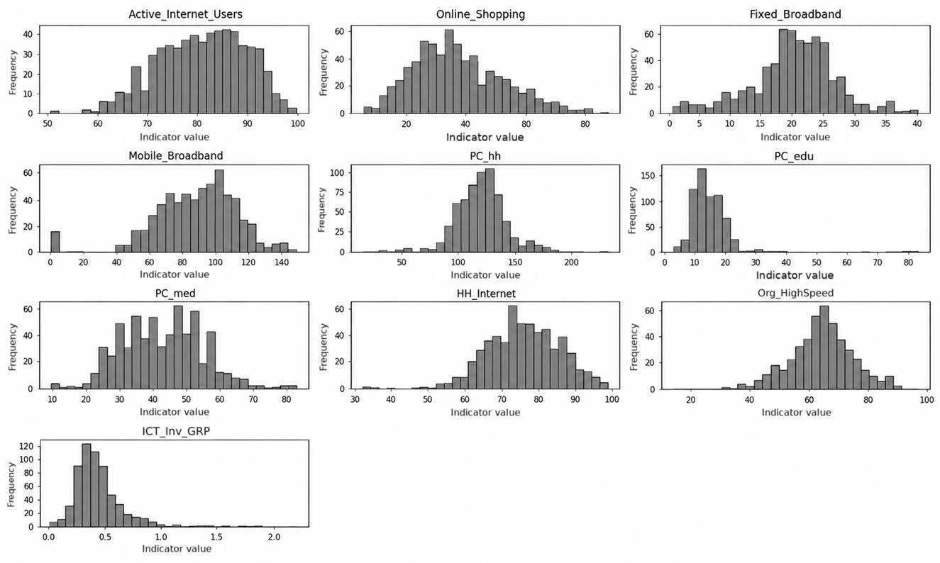
Figure 1 - Distribution of the Data

Source: compiled by the authors

The correlation analysis (Figure 2) showed that not pairwise correlation coefficient exceeded 0.70. Although this does not eliminate all conceptual overlap among indicators, it suggests that no pair of variables is strongly linearly associated.

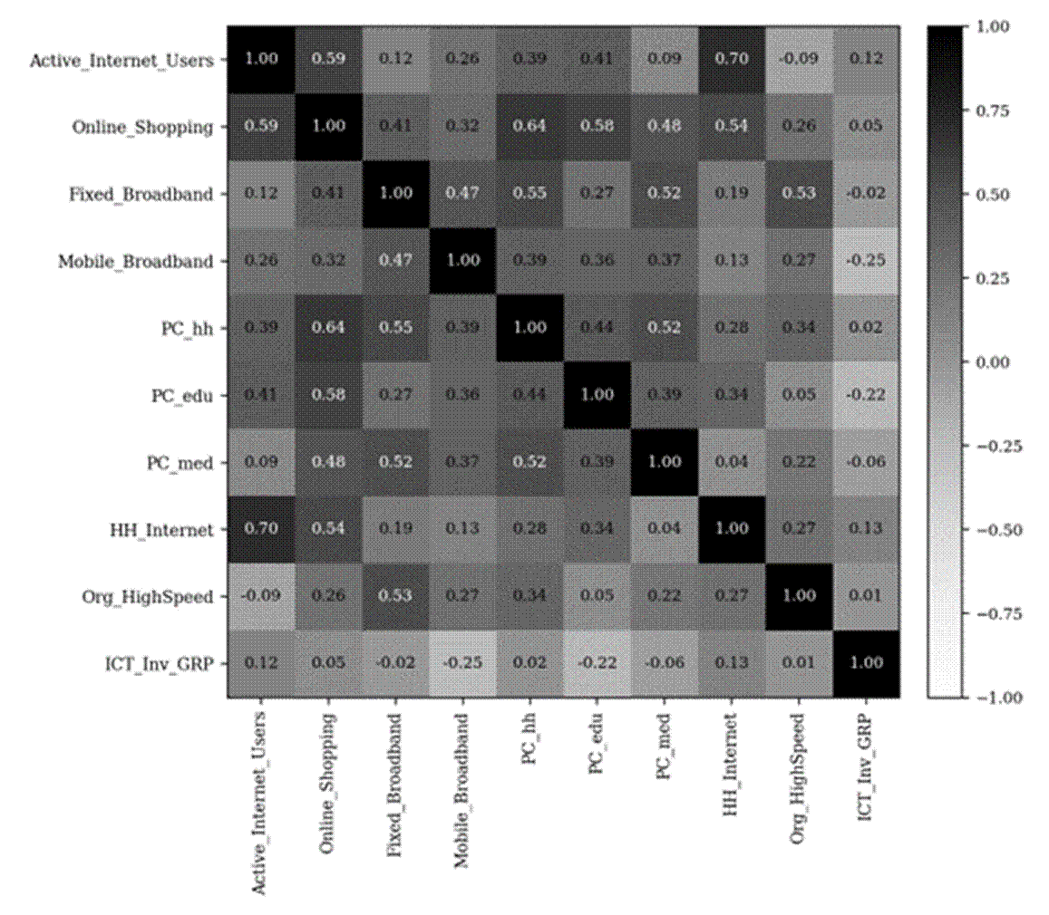
Figure 2 - Pearson correlation matrix averaged over 2016-2023

Source: compiled by the authors

To obtain valid cluster analysis results, the data are first normalized in order to bring the features to a comparable scale. This step is necessary because features measured in larger units may artificially dominate features with a smaller scale, which distorts the results. In this study, normalization was performed using the Min-Max method, which transforms feature values into a single range from 0 to 1.

Stage 4. Modelling. The normalized features for 2023 were used to compare candidate algorithms and to select a parsimonious and interpretable number of clusters. The final choice was based on a combined assessment of internal validation metrics, the stability of the solution, and the substantive interpretability of the resulting regional profiles. Analyzing a single year made it possible to assess relative differences between regions correctly and to determine the model parameters, which were then applied to the data for other periods to study the structure and dynamics of the clusters.

The dendrogram (Figure 3) suggests a possible split into 3-4 groups of regions, which is consistent with the elbow method (Figure 4), where the reduction in within-cluster error becomes less pronounced after 3–4 clusters.

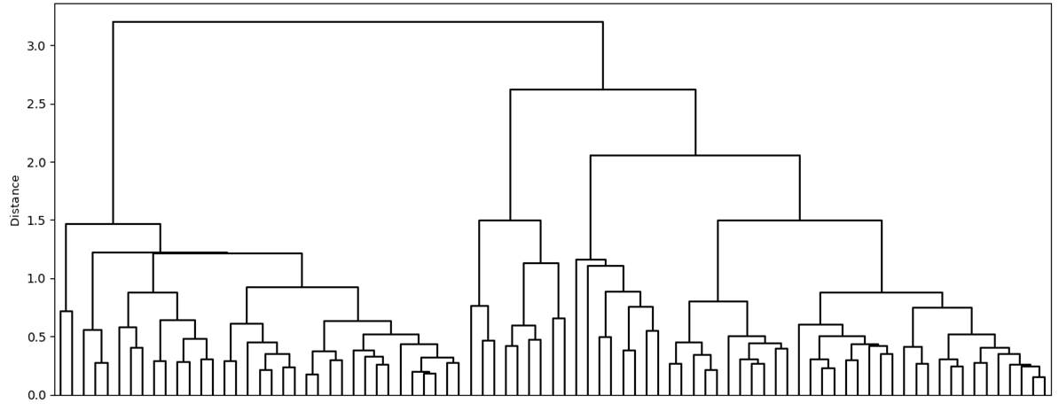
Figure 3 – Dendrogram

Source: calculated by the authors

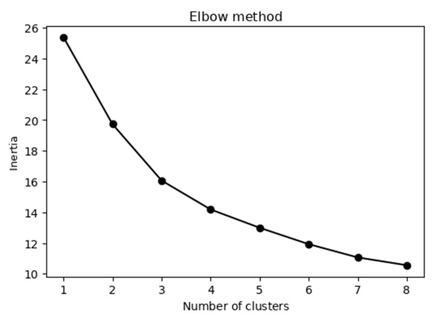
Figure 4 - Elbow method

Source: calculated by the authors

Accordingly, algorithms requiring the number of clusters to be specified in advance were run with three and four clusters. For the remaining algorithms, hyperparameters were tuned to obtain high values of the quality metrics while preserving the substantive interpretability of the identified clusters.

Stage 5. Evaluation. The results of the cluster analysis are presented in Table 3.

Table 3 - Quality of regional clustering based on 2023 data

The algorithm comparison led to the following findings:

- GMM achieved the highest silhouette coefficient; however, its lower Calinski–Harabasz index and higher Davies–Bouldin index indicate that the quality metrics do not identify a single unequivocally superior solution.

- Mean Shift identified only two clusters. Despite its high silhouette coefficient, such a partition does not meet the objective of identifying several groups of regions and complicates their substantive interpretation.

- k-means, BIRCH, and Spectral Clustering produced comparable results. K-means was selected as the main algorithm because it produced a stable and readily interpretable three-cluster solution. This choice reflects a combined methodological assessment rather than uniform superiority across all validation metrics.

The density-based algorithms (DBSCAN, HDBSCAN, and OPTICS) did not reveal a stable structure: under all tested settings, they either assigned most regions to noise or merged them into a single cluster, and they were therefore excluded from further comparison. It is likely that the regions do not form dense, isolated concentrations but rather a continuum with blurred boundaries.

The k-means algorithm was applied separately for each year. The clustering results (Table 4) confirm that the choice of three clusters is justified. Thus, a substantively interpretable three-cluster solution was obtained for every year of the study period. In some years, a four-cluster solution performed better according to an individual metric; therefore, the preference for three clusters reflects the combined evaluation criterion.

Table 4 – Results of k-means clustering

Since the cluster numbers assigned by the algorithm are arbitrary and may differ between years, a rank ordering of the clusters was introduced to ensure comparability of the results; it was calculated from the mean values of the original indicators in each cluster. Rank 0 corresponds to the most developed regions and rank 2 to the least developed.

Stage 6. Deployment: interpretation, visualization, and recommendations. To achieve the objective of the study, the clustering results were analyzed using the mean indicator values for the period under consideration (Table 5).

Table 5 - Description of the clusters

On this basis, standardized cluster profiles were constructed (Figure 5).

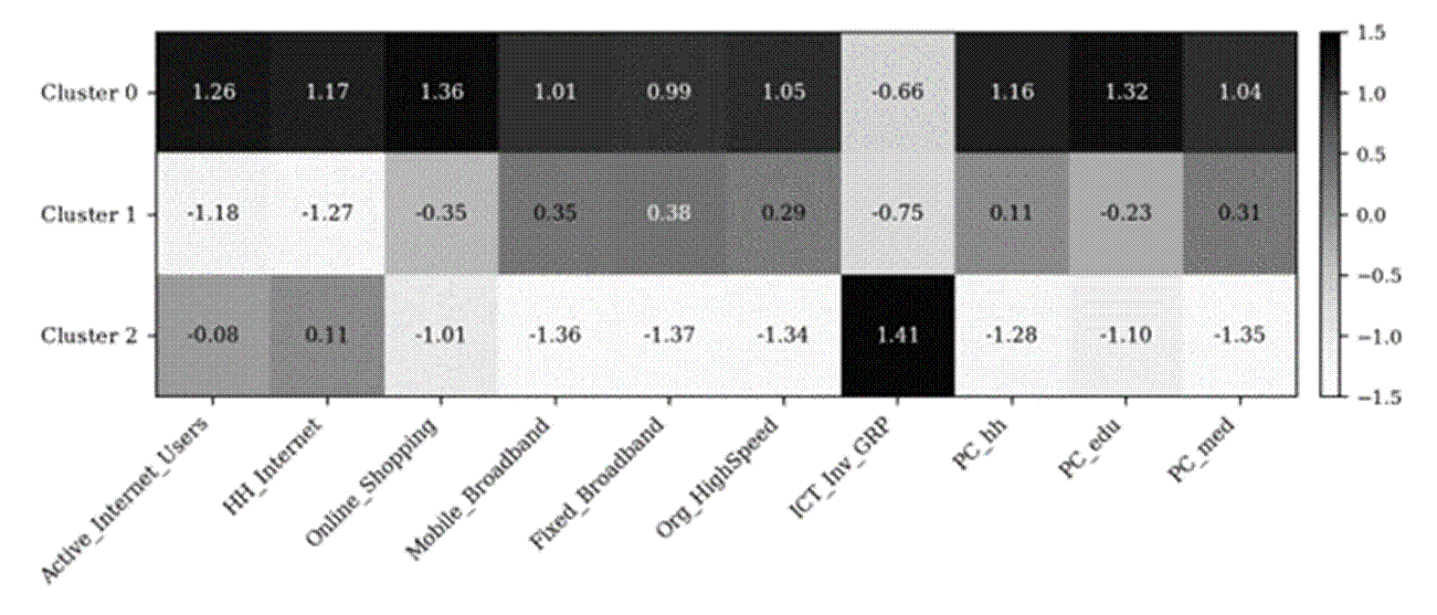
Figure 5 - Cluster profiles (compiled by the authors)

Source: calculated by the authors

Cluster 0 (digital development leaders) is characterized by the highest values on nearly all indicators. Its share of ICT investment in GRP is relatively low. This pattern may reflect a mature infrastructure base, differences in regional investment structures, or measurement characteristics and therefore requires cautious interpretation. Cluster 1 (regions with relatively low digital engagement) is in the middle on most indicators. Its distinctive feature is the lowest share of active Internet users and of households with Internet access among the three clusters. Cluster 2 (infrastructure-constrained regions) stands out for very low availability of fixed and mobile broadband. At the same time, it has the highest share of ICT investment in GRP.

Running the cluster analysis separately for each year made it possible to assess the stability of the cluster structure over time. It also allowed us to distinguish two groups of regions by the stability of their cluster membership: those that remained in the same cluster and those that changed clusters during the study period. The list of stable regions is given in Table 6.

Table 6 - Regions with stable digital development

The dynamics of cluster membership for the remaining regions is shown in Figure 6.

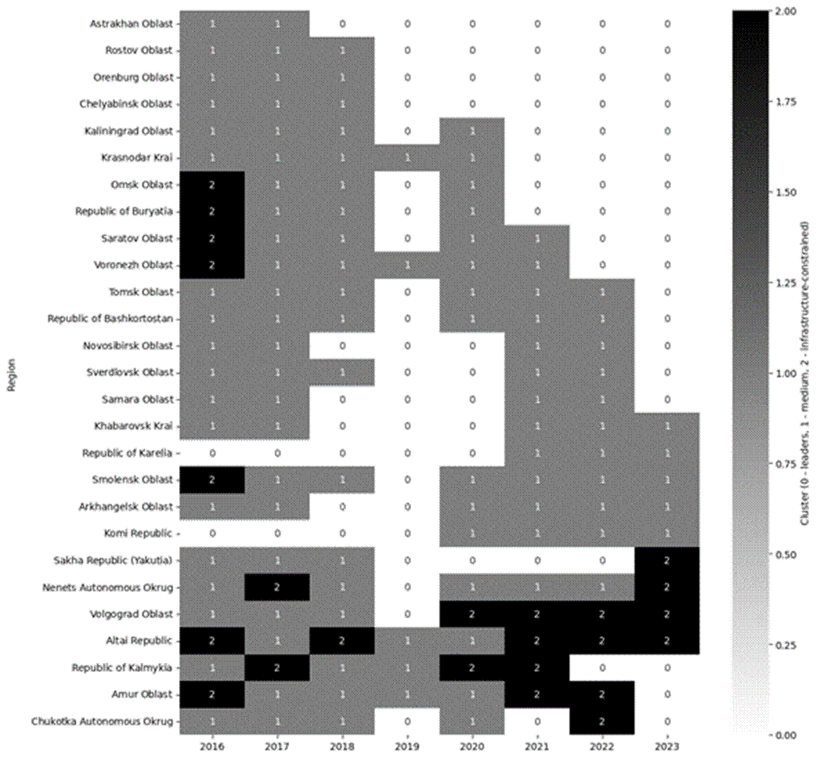
Figure 6 - Dynamics of unstable regions

Source: compiled by the authors based on their own calculations

When analyzing the dynamics of cluster transitions, the following points deserve attention:

1 The largest number of transitions of regions from Cluster 1 to Cluster 0, i.e., from the intermediate group to the group of leaders, was observed in 2019. This increase coincided with the launch of the national project “Digital Economy” in the same year. However, this temporal coincidence does not establish a causal relationship and should be interpreted cautiously.

2. A region's transition to a cluster with a lower rank does not mean an absolute deterioration of its indicators. Owing to the cross-sectional normalization of the data, such a change should be interpreted as a slower pace of development compared with other regions.

Next, the SHAP library was used to visualize the features that contribute most and least to the formation of the cluster groups (Figure 7). The most significant features were the shares of active Internet users and of households with Internet access, as well as the availability of mobile and fixed broadband access.

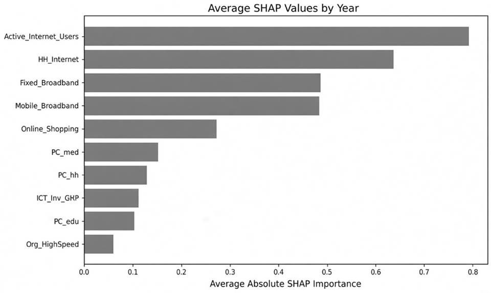
Figure 7 – Contribution of features to the differences between clusters

Source: compiled by the authors based on their own calculations

To assess whether the original set of features could be reduced, clustering was repeated using the four indicators identified above.

Applying the k-means algorithm with k = 3 to the four indicators for 2023 produced higher internal clustering scores with a reduced indicator set: the silhouette coefficient increased from 0.21 to 0.36, the Calinski–Harabasz index from 23.8 to 52.1, and the Davies–Bouldin index decreased from 1.49 to 1.01. At the same time, 10 of the 85 regions (12%) changed cluster membership, which confirms that the results obtained with the reduced set of indicators are comparable and justifies its further use.

The availability of data on the four selected indicators for 2024–2025 made it possible to construct an exploratory extension of the analysis for these years. The k-means algorithm (k=3) was applied to the data for these years. Because the 2024–2025 analysis uses a reduced indicator set, its results should be interpreted as broadly comparable with, but not identical to, the full 2016–2023 classification. The clustering results are shown on maps of the constituent entities of the Russian Federation, with regions distributed by cluster (Figures 8–9).

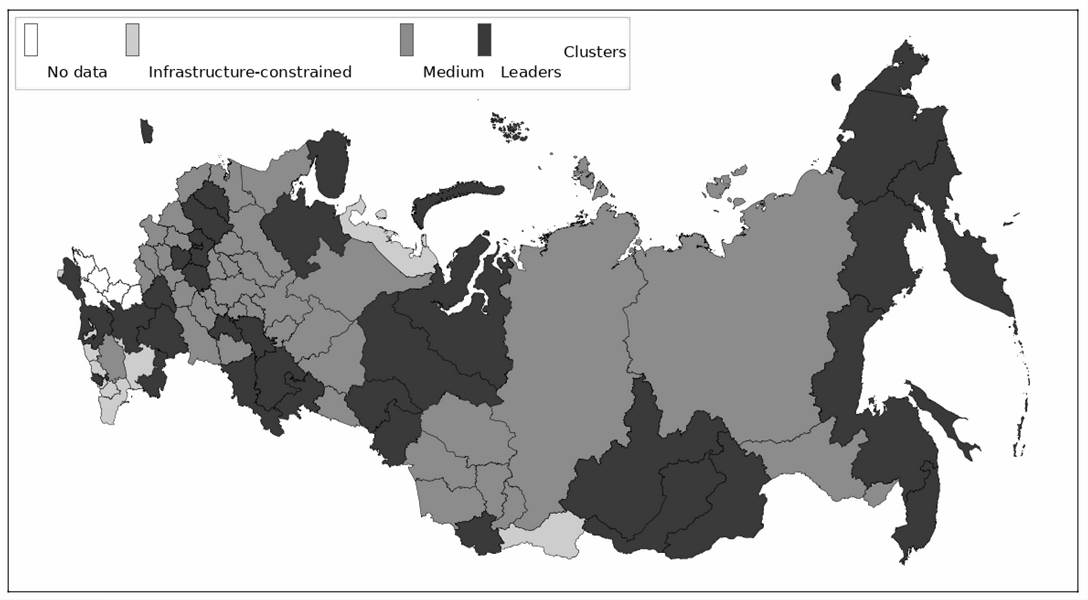
Figure 8 - Regional digital development map, 2024

Source: compiled by the authors based on their own calculations

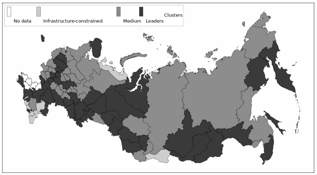
Figure 9 - Regional digital development map, 2025

Source: compiled by the authors based on their own calculations

The results make it possible to tailor digital policy to regional conditions. For regions with low digital engagement among the population (Cluster 1), the priority is to build digital skills and encourage the use of online services. The problem often lies in limited familiarity with digital technologies and distrust of the online environment, so free digital literacy programs should be expanded, with particular attention to rural residents and older people.

Regions with weak infrastructure (Cluster 2) first of all need a wider telecommunications network and broader use of modern digital technologies, including next-generation mobile networks (4G/5G), satellite Internet, and fiber-optic lines. State support matters here as well. Infrastructure projects are expensive, and without public funding for digital development in remote regions is likely to be slow. Therefore, subsidies and tax incentives for companies that build and upgrade digital infrastructure would help.

Leading regions (Cluster 0) mainly need to keep their positions and share their experience with other territories.

Discussion

The results support the expectation that Russian regions differ substantially in their relative level of digital development. The resulting typology is generally consistent with the findings of earlier studies. As the study closest to the present one, it is worth noting the work [5], in which the constituent entities of the Russian Federation were also clustered by digital development indicators using panel data (2010–2018), and clustering algorithms (k-means, BIRCH, DBSCAN) were compared, with the most suitable one selected on the basis of quality metrics.

The present study extends earlier regional typologies by comparing a broader set of clustering algorithms, analysing annual changes in cluster membership from 2016 to 2023, and providing an exploratory update for 2024–2025 based on a reduced set of indicators.

The main limitation of this study is the quality and availability of the source statistical data. Because some indicators are based on statistical surveys, the values obtained may be affected by the way the sample was constructed. The reliability of respondents' answers may also affect the results. Another limitation is the lack of regional breakdowns for the indicators specified in the passports of national projects and used to monitor progress toward digital transformation goals. These indicators are published only at the level of the Russian Federation, without a breakdown by constituent entity, which limits their use in regional analysis. A further limitation is that the clustering results depend on the selected indicators, the scaling procedure, and algorithmic settings. The proposed typology should therefore be interpreted as an empirically grounded representation of regional digital differentiation rather than as a definitive classification.

Given the identified heterogeneity of the groups of regions, a promising direction for further research is to build regression models within each cluster. This would make it possible to assess the impact of digital transformation on the population's standard of living. Household consumer expenditure could serve as an indicator of living standards. An alternative is to use a measure of population satisfaction with quality of life. Such a measure could be based on official household surveys, administrative statistics, and, where appropriate, carefully validated alternative data sources.

Conclusion

Today, digital development is becoming increasingly important for the economies of countries around the world, and Russia is no exception. Digital transformation has been established as one of the country's key strategic development goals. However, Russian regions differ in their socio-economic conditions, which should be taken into account when developing digital policy measures. This served as the basis for the present study. The aim was to identify groups of Russian regions with a similar level of digital development using methods of multivariate statistics and cluster analysis.

To achieve this aim, the study was conducted following the main stages of the adapted CRISP-DM methodology. The statistical data were drawn from the official portals of Rosstat and UISIS.

To select a clustering method, various algorithms and quality metrics were compared. Based on the comparison, the k-means algorithm was chosen, for which a partition into three clusters was found to be optimal.

As a result, the findings support the study’s expectation that Russian regions differ in their relative level of digital development. The cluster analysis revealed a digital divide between Russian regions and made it possible to identify three groups of regions that differ in their level of digital transformation. Using the SHAP library, the most significant indicators were determined, and on their basis additional clustering was carried out for 2024–2025. These findings provide an empirical basis for tailoring digital policy to the specific needs of each cluster. The practical significance of the study lies in the possibility for regional authorities to use the results when designing and adjusting digital policy measures to ensure the sustainable development of the regions.