Влияние мировых цен на нефть и других факторов на ВВП Катара за период I квартал 2003 – IV квартал 2023

The importance of research

The importance of the research stems from the fact that the impact of international oil prices and some factors on the Qatari GDP has a significant impact on the Qatari economy, negatively or positively, as in the event of a rise in global oil prices, it gives a positive signal for an improvement in the GDP in Qatar.

The research problem

Although the State of Qatar occupies an advanced position in the world in gas production, as well as being ranked first in the Arab countries in gas production, it is also an oil-producing state that produces and exports oil, and this means an increase in the state’s public revenues through which it covers public expenses. Completely and successfully, the availability of such revenues helps the Qatari state develop its infrastructure so that it becomes prosperous for the Qatari economic reality.

The Hypothesis research

The research hypothesis is based on the vision that “the rise in global oil prices leads to increases in oil imports and thus an increase in the Qatari gross domestic product.”

Research objective

Standard analysis of world oil prices, oil exports, oil production, and analysis of the country’s gross domestic product using quantitative methods according to the assumptions of economic theory.

Research methodology and structure:

The researcher relied on the standard approach adopted in studies of the impact of international oil prices and some factors on the Qatari gross domestic product

This is done by analyzing the available data about the research problem and the purpose of its study.

the introduction

The rentier characteristic is one of the most important features that characterize the Arab Gulf economies, given that they possess a source of rentier revenues, natural resources, and reserves, and the Qatari economy is one of these economies. In general, the aforementioned economies can be classified into two types. The first is that some Gulf economies were able to record remarkable development leaps, such as the economy. Saudi Arabia, Qatar, and the UAE compared to the second type, which are economies that still depend mainly on revenues generated from the oil sector, and it can be said that these economies revolve in a vicious circle of rentierism.، However, the Qatari economy was able, in record periods, to record clear developments in local and even international arenas, at the level of sporting activities and events, and hosting international tournaments and the World Cup. Despite Qatar’s small area, it enjoys latent natural resources, in addition to the huge oil and natural gas reserves, which can be developed. The oil and natural gas industry came gradually since the discovery of these resources in the middle of the twentieth century, as the state was able, through strategic plans, to diversify its sources of income as well as maintain the sustainability of these wealth and natural resources, as they are not only for the current generation, but also to preserve the share of future generations in them.، Diversification strategies include other multiple sectors, such as education, tourism, and the use of advanced technology. Qatar’s adoption of successful development and economic policies enhances the advanced reality of the economy, especially as it now seeks to stimulate entrepreneurship and innovation cycles, as well as assigning and supporting areas of research and development not only on the local scene, but also on the international arena. Regional and international.

Data

The World Bank data is considered the main source of our data in the current research, but this data has been divided into quarterly or quarterly data, which is a statistical procedure that is used to enhance the sample size and work to increase it according to standard frameworks in order to obtain logical and realistic estimates, avoid falling, and solve regression or Pseudo integration between the research variables studied, and the GDP variable was used as a dependent variable, while the oil exports variable OIL_EXP, oil production OIL_PRO, and the world oil prices variable W_OIL_PRI are exogenous variables. Thus, it can be said that the relationship of the dependent variable to the independent variables is a multiple regression relationship, and the studied time series extended from one quarter The first for the year 2003 to the fourth quarter of 2023 as follows:

Table (1) World oil prices, oil exports, oil production, natural gas for Qatar (2023Q4 - 2003Q1)/dollar

Pretests

Therefore, to determine the appropriate details for the lighting reality, the research must have some control over its statistical indicators and determine them. We begin this group by testing the wind histogram [8, GERASKIN, Petr; FANTAZZINI, 2020]^. First, unit root tests [1, Ayman Al-Aashoush2017] Secondly, of course, unit root tests are divided into two parts, the first is the expanded Dickey-Fuller test [14, Sahab Al-Samadi; Ahmed Malawi,2015] The second is the Phillips-Perron test [6, Farid Al-Jaouni; Ahmed Al-Ali; Alaa Abdullah Al-Dheeb,2013] For the unit root, after this stage we can choose the optimal methodology that matches the nature and sample of the research, as follows:

A- Chart

It appears from Chart (1) that all variables suffer from the problem of instability [10, KAN, Man Shan; TAN, Andy CC; MATHEW, Joseph ,2015] And stillness, some of them suffer from the problem of trend over time, and others suffer from the average, as in the following diagrams:

Chart (1): International oil prices, oil exports, oil production, natural gas for Qatar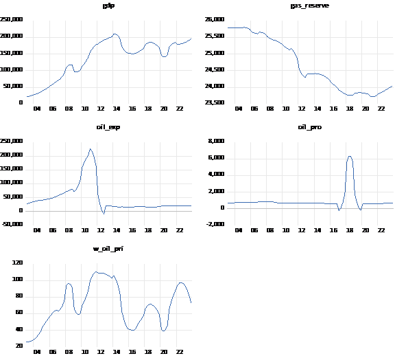

Source: Outputs of the statistical program Eviews 12.0

B-Unit root tests( 15 SCHWERT, G. William,2002 )

Unit root tests are classified as pre-tests to choose the appropriate model for the nature and methodology of the study and the research variables. Here two unit root tests were used, the first test is the expanded Dickey-Fuller test. [5, CANER, Mehmet; HANSEN, Bruce,2001] The other test is the Phillips-Perron test [3, BREITUNG, Jörg; FRANSES, Philip Hans,1998] We notice from the following table and the resulting results that all variables did not stabilize at the level because their probability value exceeds 5%, except for the oil production variable, Feller which stabilized at the level of 5%. Therefore, the first difference must be taken for these variables, and indeed the first difference was taken for them and they stabilized at The one% level at all, and successively, the research data and its variables were tested and subjected to the expanded Dickey-Feller unit root test, which showed consistency in terms of results with the Philips-Perron test. In general, the test results indicate that all the research variables did not stabilize at the level because they came with a probability of more than 5%. With the exception of the oil production variable, the first difference was also taken and the results were included in the following table:

Table 2: Unit root tests for the expanded Dickey- and Phelps-Perron

Methodology

By following stability tests according to the Graphs test for each of the world oil prices, oil exports, oil and natural gas production, as well as the unit root tests, expanded Died-Feller and Phelps-Perron, in accordance with the results of the graph, it is most likely observed that the variables will not stabilize at the level except for one variable, which is oil production. This makes it necessary for us to choose the appropriate methodology for this type of quiescence. It can be said that this type of quiescence, in which the levels of stability are distributed between the level and the first difference, is compatible with the autoregressive methodology for slow distributed gaps. ARDL [17, SARI, Ramazan; EWING, Bradley T.; SOYTAS, Ugur,2008] The model can be written in its general form [12, PINN, Stan Lee Shun,2011] As follows:

Yt=a0+a1yt-1+a2yt-2+---+apyt-p+B0Xt+B1Xt-1+B2Xt-2+---+BqXt-q+ Ƹt

whereas

Yt= variable

Xt= independent variable 123 ----- n

T = time

aO,aI,a2,-----,ap=Historical coefficients of change

Bo,B1,B2,----,Bg= independent time variation coefficients

Ƹt=random error

Top of Form

whereas

Y t=dependent variable

Xt=the independent variable

T=time

ao,a1,a2,----,ap=time delay coefficients of the dependent variable

BO,B!,B2,----,Bq=time delay coefficients of the independent variable

Ƹt=random error

It is worth noting that the distributed lag autoregressive methodology is consistent with the nature of the study variables and that it is compatible with variables whose levels of rest range between the level and the first difference. This methodology is based on two basic pillars: the first is testing the limits. [18, TANEJA, Sanjay, et,2023] Bound test، The second is the integration parameter [16, SHAHBAZ, Muhammad; RAHMAN, Mohammad Mafizur,2010] Co-integration Equation It must be negative and significant at the same time. The test results are listed in the following table:

Table 3: Methodology ARDL

Posttests

Firstly: AKAIKE INFORMATION CRITERIA TEST [ 9, HU, Shuhua. Akaike ,2007] There is no doubt that we cannot go beyond the Akaike test (longitudinal wave), which is at the forefront of these tests, and the nature of this test is based on comparison with the best 20 models in terms of statistical and measurement characteristics, and the model proposed by (2 ,0,0,0,2) ARDL is the best, and this indicates that the GDP has two slowdowns and no slowdown for the natural gas variable, oil exports, and oil production, and two slowdowns for global oil prices, as follows::

Scheme (2) Akaik test

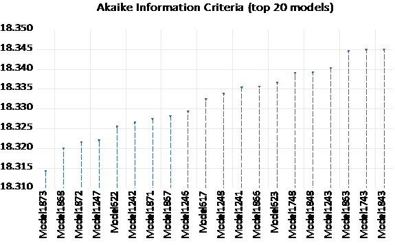
Source: Outputs of the statistical program Eviews 12.0

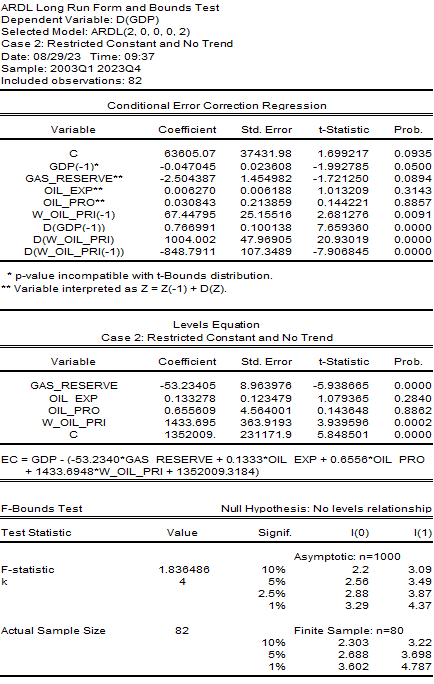
secondly: ARDL BOUND TEST

The results of the analysis of the bounds test for the ARDL methodology showed that there is no long-term balanced relationship between the independent research variables and the dependent variable, which is the gross domestic product, since the value of F-CALCU, which is 1.8, is less than all the upper and lower limits for the significance levels of 1%, 5%, 10%, and 2. 5%. Therefore, it can be said that there is no long-term balanced relationship between the research variables mentioned above, as in the following table:

Schedule (4) ARDL BOUND TEST

Source: Outputs of the statistical program Eviews 12.0

Third: ARDL LOUNG RUN COINTEGRATION (11 NKORO, Emeka, et,2016 ) The cointegration equation shows the complementary relationships between external variables and the GDP. This relationship showed that there is a negative relationship between the natural gas reserves variable and the GDP, which is somewhat smooth and logical because an increase in storage in a variable or an increase in natural gas will negatively affect Gross Domestic Product (GDP) is one of the sources of financing that the State of Qatar relies on mainly through the export of natural gas to Europe. And vice versa, if this reserve is reduced, it will be reflected positively on the GDP, which is a logical economic relationship. As for the other variables, which are both oil exports and oil production, as well as global oil prices, they have a direct impact on the GDP index, and they are relationships at the core of the region. Economic because when it increases, this will lead to an increase in the gross domestic product by the amount or parameter value of the variables mentioned as below:

Fourthly: Coint-Equation

The parameter of the cointegration equation must be negative and significant at the same time. The ARDL error correction test showed this by being negative and significant, meaning that its probability value is less than 5%. The error correction parameter indicates that the line can be corrected by about 1.42, that is, approximately within six months. As below or as in the following table:

Table (5) Error correction parameter

Fifth: LM Test [2,BALTAGI, Badi H.; JUNG, Byoung Cheol; SONG, Seuck Heun, 2010] The Breusch-Godfrey serial correlation test shows that the selected model does not suffer from the problem of serial correlation between random residuals, since the probability value for both F-CALCL and Chi-Square is greater than 5%, as in the following table:

Schedule (6) Breusch-Godfrey Serial Correlation LM Test

Sixth: Homogeneity of variance test

The test shows non-stationarity of homogeneity of variance Heteroskedasticity Test [7, GLEJSER, Herbert,1969] The selected model does not suffer from this problem, but rather it is characterized by stable homogeneity of variance Homoscedasticity [4, BUCHINSKY, Moshe,1998] being that F-CALCL و Chi-Square It is 5% as in the following table:

Schedule (7) Heteroskedasticity Test

The cumulative sum test indicates that the behavior of the studied series is normal and does not suffer from distortions, as it proceeds within the two critical limits, with a significance level of 5%, and this is a good indicator. As for the cumulative sum squares index, it shows a violation of the critical limits in the path of the phenomenon, and this is the result of a number of causes. Among them, there may be a distortion in the data of one of the model variables, or some of these data may be estimated, unreal, or illogical, or we may attribute this to other reasons that cannot be limited to this point, but in general, the parameters of the estimated model are good and have shown agreement. With economic logic, the model in its comprehensive form does not suffer from statistical or measurement problems and has passed all these tests successfully, as shown below:

The variation in the stationarity of the studied variables and their distribution between the level and the first difference, their stationarity at the first difference, and the variables not exceeding the second difference led to the choice of the autoregressive methodology for slowed and distributed gaps (ARDL), and the optimal slowdown was chosen as follows (2, 0, 0, 0, 2), that is, two slowdowns. For the dependent variable, which is the gross domestic product, and without slowing down for the independent variables, which are, respectively, natural gas reserves, oil exports, and oil production, in addition to two slowdowns for global oil prices.، This set of slowdowns was chosen according to a scientific methodology based in its interpretation on the Akaike criterion, which is considered the ideal standard for recording the lowest values ​​of the parameters of the estimated model. As the Akaike test shows, the model that we mentioned previously was chosen from among 20 estimated models, and for different slowdowns. As for With post-tests, starting with the limits test, which showed us that there are no long-term complementary relationships between external variables and GDP, since the value of F-CALCL is less than the minimum limits for all levels: 1%, 5%, 2.5%, 10%, as it reached 1.84.، The same is true for the error correction parameter, which has proven its quality, and it is a parameter with a negative value and a significance at the same time, as in Table (5). In addition to the post-tests, the LM test is considered an autocorrelation test for random residuals, which states that there is no problem of autocorrelation between random residuals. The fact that the probability value exceeds 5%, as is the case with the non-stationarity of homogeneity test, which shows that there is no problem of non-stationarity of homogeneity of variance. Rather, the model is in a state of constant homoscedasticity for the same previous reason. The post-tests were concluded by testing the cumulative sum and the squares of the cumulative sum.، If the first test shows normal behavior for the path of the phenomenon and its estimated model, the second test shows that there is a deviation in the path of the estimated phenomenon because the path of the phenomenon has recorded a departure from the two critical limits. Some of the reasons for this have been mentioned above..

References:

Ayman Al-Aashoush (2017). Unit root tests for panel data (first generation tests) applied to a sample of developing countries Tishreen University Journal-Economic and Legal Sciences Series.
Baltagi Badi H., Jung Byoung Cheol, Song Seuck Heun (2010). Testing for heteroskedasticity and serial correlation in a random effects panel data model Journal of Econometrics.
Breitung Jörg, Franses Philip Hans (1998). On Phillips–Perron-type tests for seasonal unit roots Econometric Theory.
Buchinsky Moshe (1998). Recent advances in quantile regression models: a practical guideline for empirical research Journal of human resources.
Caner Mehmet, Hansen Bruce E. (2001). Threshold autoregression with a unit root Econometrica.
Farid Al-Jaouni, Ahmed Al-Ali, Alaa Abdullah Al-Dheeb (2013). Analysis of the relationship between the general budget and the trade balance using the method of cointegration and causality, an applied study on the Syrian economy during the period 1990-2009 Tishreen University Journal-Economic and Legal Sciences Series.
Geraskin Petr, Fantazzini Dean (2020). Everything you always wanted to know about log-periodic power laws for bubble modeling but were afraid to ask. New Facets of Economic Complexity in Modern Financial Markets
Glejser Herbert (1969). A new test for heteroskedasticity Journal of the American Statistical Association.
Hu Shuhua (2007). Akaike information criterion
Kan Man Shan, Tan Andy C.C., Mathew Joseph (2015). A review on prognostic techniques for non-stationary and non-linear rotating systems Mechanical Systems and Signal Processing.
Nkoro Emeka, et al. (2016). Autoregressive Distributed Lag (ARDL) cointegration technique: application and interpretation Journal of Statistical and Econometric methods.
Pinn Stan Lee Shun, et al. (2011). Empirical analysis of employment and foreign direct investment in Malaysia: An ARDL bounds testing approach to cointegration Advances in Management and Applied Economics.
Ploberger Werner, Krämer Walter (1990). The local power of the CUSUM And CUSUM of squares tests Econometric Theory.
Sahab Al-Samadi, Ahmed Malawi (2015). The impact of government taxes on the performance of the Amman Stock Exchange: an autoregressive distributed lag (ARDL) model
Sari Ramazan, Ewing Bradley T., Soytas Ugur (2008). The relationship between disaggregate energy consumption and industrial production in the United States: an ARDL approach Energy Economics.
Schwert G. William (2002). Tests for unit roots: A Monte Carlo investigation Journal of Business & Economic Statistics.
Shahbaz Muhammad, Rahman Mohammad Mafizur (2010). Foreign capital inflows-growth nexus and role of domestic financial sector: an ARDL co-integration approach for Pakistan Journal of Economic Research.
Taneja Sanjay, et al. (2023). India’s total natural resource rents (NRR) and GDP: An augmented autoregressive distributed lag (ARDL) bound test Journal of Risk and Financial Management.
Страница обновлена: 27.05.2025 в 05:27:17